Basic Mathematics for Economists phần 4 pdf

Appendix: linear programming
Although basically an extension of the linear algebra covered in the main body of this chapter,
the technique of linear programming involves special features which distinguish it from other
linear algebra applications. When all the relevant functions are linear, this technique enables
one to:
• calculate the profit-maximizing output mix of a multi-product firm subject to restrictions
on input availability, or
• calculate the input mix that will minimize costs subject to minimum quality standards
being met.
This makes it an extremely useful tool for managerial decision-making.
However, it should be noted that, from a pure economic theory viewpoint, linear pro-
gramming cannot make any general predictions about price or output for a large number of
firms. Its usefulness lies in the realm of managerial (or business) economics where economic
techniques can help an individual firm to make efficient decisions.
Constrained maximization
A resource allocation problem that a firm may encounter is how to decide on the product mix
which will maximize profits when it has limited amounts of the various inputs required for
the different products that it makes. The firm’s objective is to maximize profit and so profit
is what is known as the ‘objective function’. It tries to optimize this function subject to the
constraint of limited input availability. This is why it is known as a ‘constrained optimization’
problem.
When both the objective function and the constraints can be expressed in a linear form
then the technique of linear programming can be used to try to find a solution. (Constrained
optimizationofnon-linearfunctionsisexplainedinChapter11.)Weshallrestricttheanalysis
here toobjective functions which have onlytwo variables, e.g. when onlytwo goods contribute
to a firm’s profit. This enables us to use graphical analysis to help find a solution, as explained
in the example below.
Example 5.A1
A firm manufactures two goods A and B using three inputs K, L and R. The firm has at its
disposal 150 units of K, 120 units of L and 40 units of R. The net profit contributed by each
unit sold is £4 for A and £1 for B. Each unit of A produced requires 3 units of K, 4 units of L

plus 2 units of R. Each unit of B produced requires 5 units of K, 3 units of L and none of R.
What combination of A and B should the firm manufacture to maximize profits given these
constraints on input availability?
Solution
From the per-unit profit figures in the question we can see that the linear objective function
for profit which the firm wishes to maximize will be
π = 4A + B
where A and B represent the quantities of goods A and B that are produced.
© 1993, 2003 Mike Rosser
(R)
X
(K)
(L)
0
A30 50

40

80

*
B
30
40
20
13
Figure 5.A1
The total amount of input K required will be 3 for each unit of A plus 5 for each unit of B
and we know that only 150 units of K are available. The constraint on input K is thus
3A + 5B ≤ 150 (1)

Similarly, for L
4A + 3B ≤ 120 (2)
and for R
2A ≤ 40 (3)
As the firm cannot produce negative quantities of the two goods, we can also add the two
non-negativity constraints on the solutions for the optimum values of A and B, i.e.
A ≥ 0(4)
and
B ≥ 0 (5)
Now turn to the graph in Figure 5.A1 which measures A and B on its axes. The first step
in the graphical solution of a linear programming problem is to mark out what is known
as the ‘feasible area’. This will contain all the values of A and B that satisfy all the above
constraints (1) to (5). This is done by eliminating the areas which could not possibly contain
the solution.
We can easily see that the non-negativity constraints (4) and (5) mean that the solution
must lie on, or above, the A axis and on, or to the right of, the B axis.
To mark out the other constraints we consider in turn what would happen if the firm entirely
used up its quota of each of the inputs K, L and R. If all the available K was used up, then in
constraint (1) an equality sign would replace the ≤ sign and it would become the function
3A + 5B = 150 (6)
© 1993, 2003 Mike Rosser
Thislinearconstraintcaneasilybemarkedoutbyjoiningitsinterceptsonthetwoaxes.When
A=0thenB=30andwhenB=0thenA=50.Thustheconstraintwillbethestraight
linemarked(K).Thisisratherlikeabudgetconstraint.IfalltheavailableKisusedthen
thefirm’sproductionmixwillcorrespondtoapointsomewhereontheconstraintline(K).
Itisalsopossibletouselessthanthetotalamountavailable,inwhichcasethefirmwould
produceacombinationofAandBbelowthisconstraint.Pointsabovethisconstraintarenot
feasible,though,astheycorrespondtomorethan150unitsofK.
Inasimilarfashionwecandeducethatallpointsabovetheconstraintline(L)arenot
feasiblebecausewhenalltheavailableLisusedupthen

4A+3B=120(7)
TheconstraintonRisshownbytheverticalline(R)sincewhenallavailableRisusedupthen
2A=40(8)
Pointstotherightofthislinewillnotbefeasible.
Havingmarkedouttheindividualconstraints,wecannowdelineatetheareawhichcontains
combinationsofAandBwhichsatisfyallfiveconstraints.Thisisshownbytheheavierblack
linesinFigure5.A1.
Weknowthatthefirm’sobjectivefunctionisπ=4A+B.Butaswedonotyetknow
whattheprofitis,howcanwedrawinthisfunction?Toovercomethisproblem,firstmake
upafigureforprofit,whichwhendividedbythetwoper-unitprofitfigures(£4and£1)will
givenumberswithintherangeshownonthegraph.Forexample,ifwesupposeprofitis£40,
thenwecandrawinthebrokenlineπ
40
correspondingtothefunction
40=4A+B
Ifwehadchosenafigureforprofitofmorethan£40thenwewouldhaveobtainedaline
parallel to this one, but further away from the origin; e.g. the line π
80
corresponds to the
function 80 = 4A + B.
If the firm is seeking to maximize profit then it needs to find the furthest profit line from
the origin that passes through the feasible area. All profit lines will have the same slope and
so, using π
40
as a guideline, we can see that the highest feasible profit line is π∗ which just
touches the edge of the feasible area at X. The optimum values of A and B can then simply
be read off the graph, giving A = 20 and B = 13 (approximately).
A more accurate answer may be obtained algebraically, once the graph has been used to
determine which is the optimum point, since the solution to a linear programming problem
will nearly always be at the intersection of two or more constraints. (Exceptionally the

objectivefunctionmaybeparalleltoaconstraint–seeExample5.A3.)
The graph in Figure 5A.1 tells us that the solution to this problem is where the constraints
(L) and (R) intersect. Thus we have the two simultaneous equations
4A + 3B = 120 (7)
2A = 40 (8)
© 1993, 2003 Mike Rosser
which can easily be solved to find the optimum values of A and B.
From (8)A= 20
Substituting in (7) 4(20) +3B = 120
3B = 40
B = 13.33 (to2dp)
Thus maximum profit is
π = 4A + B = 4(20) + 13.33 = 80 + 13.33 = £93.33
The optimum combination X is on the constraints for L and R, but below the constraint for K.
Thus, as the K constraint does not ‘bite’, there must be some spare capacity, or what is often
called ‘slack’, for K. When the firm produces 20 of A and 13.33 of B, then its usage of K is
3A + 5B = 3(20) +5(13.33) = 60 +66.67 = 126.67
The amount of K available is 150 units; therefore slack is
150 − 126.67 = 23.33 units of K
Now that the different steps involved in solving a linear programming problem have been
explained let us work through another problem.
Example 5.A2
A firm produces two goods A and B, which each contribute a net profit of £1 per unit sold.
It uses two inputs K and L. The input requirements are:
3 units of K plus 2 units of L for each unit of A
2 units of K plus 3 units of L for each unit of B
If the firm has 600 units of K and 600 units of L at its disposal, how much of A and B should
it produce to maximize profit?
Solution
Using the same method as in the previous example we can see that the constraints are:

for input K 3A + 2B ≤ 600 (1)
for input L 2A + 3B ≤ 600 (2)
non-negativity A ≥ 0 B ≥ 0
ThefeasibleareaisthereforeasmarkedoutbytheheavyblacklinesinFigure5A.2.
As profit is £1 per unit for both A and B, the objective function is
π = A + B
© 1993, 2003 Mike Rosser
(L)
(K)
0
300
M
B

120
120 200
A
200
300

200

*
Figure 5.A2
If we suppose profit is £200, then
200 = A +B
This function corresponds to the line π
200
which can be used as a guideline for the slope
of the objective function. The line parallel to π

200
that is furthest away from the origin but
still within the feasible area will represent the maximum profit. This is the line π∗ through
point M. The optimum values of A and B can thus be read off the graph as 120 of each.
Alternatively, once we know that the optimum combination of A and B is at the intersection
of the constraints (K) and (L), the values of A and B can be found from the simultaneous
equations
3A + 2B = 600 (1)
2A + 3B = 600 (2)
From (1) 2B = 600 −3A
B = 300 −1.5A (3)
Substituting (3) into (2)
2A + 3(300 − 1.5A) = 600
2A + 900 − 4.5A = 600
300 = 2.5A
120 = A
© 1993, 2003 Mike Rosser
Substituting this value of A into (3)
B = 300 −1.5(120) = 120
As both A and B equal 120 then
π∗=120 + 120 = £240
The optimum combination at M is where both constraints (K) and (L) bite. There is therefore
no slack for either K or L.
It is possible that the objective function will have the same slope as one of the constraints.
In this case there will not be one optimum combination of the inputs as all points along the
section of this constraint that forms part of the boundary of the feasible area will correspond
to the same value of the objective function.
Example 5.A3
A firm produces two goods x and y which require inputs of raw material (R), labour (L) and
components (K) in the following quantities:

1 unit of x requires 12 kg of R, 10 hours of L and 15 units of K
1 unit of y requires 21 kg of R, 10 hours of L and 6 units of K
Both x and y add £200 per unit sold to the firm’s profits. The firm can use up to a total of
252 kg of R, 150 hours of L and 180 units of K. What production mix of x and y will maximize
profits?
Solution
The constraints can be written as
12x + 21y ≤ 252 (R)
10x + 10y ≤ 150 (L)
15x + 6y ≤ 180 (K)
x ≥ 0,y≥ 0
TheseareshowninFigure5.A3wherethefeasibleareaismarkedoutbytheshapeABCD0.
The objective function is
π = 200x + 200y
To find the slope of this objective function, assume profit is £2,000. This could be achieved
by producing 10 of x and none of y, or 10 of y and no x, and is therefore shown by the broken
line π
2000
. This line is parallel to the constraint (L). Therefore if we slide out the objective
function π to find the maximum value of profit within the feasible area we can see that it
coincides with the boundary of the feasible area along the stretch BC.
© 1993, 2003 Mike Rosser
(K)
(L)
B
C
(R)
0
y
12

A
D
10
12 x
30
15
10 15 21

2000
Figure 5.A3
What this means is that both points B and C, and anywhere along the portion of the
constraint line (L) between these points, will give the same (maximum) profit figure.
At B the constraints (R) and (L) intersect. Therefore these two resources are used up
completely and so
12x + 21y = 252 (1)
10x + 10y = 150 (2)
From (2)x= 15 − y (3)
Substituting (3) into (1)
12(15 − y) +21y = 252
180 − 12y + 21y = 252
9y = 72
y = 8
Substituting this value of y into (3)
x = 15 − 8 = 7
Thus profit at B is
π = 200x + 200y = 200(7) + 200(8) = £1,400 +£1,600 = £3,000
© 1993, 2003 Mike Rosser
At C the constraints (L) and (K) intersect, giving the simultaneous equations
10x + 10y = 150 (2)
15x + 6y = 180 (4)

Using (3) again to substitute for x in (4),
15(15 − y) + 6y = 180
225 − 15y + 6y = 180
45 = 9y
5 = y
Substituting this value of y into (3)
x = 15 − 5 = 10
Thus, profit at C is
π = 200x + 200y = 200(10) + 200(5) = 2,000 + 1,000 = £3,000
which is the same as the profit achieved at B, as expected. This example therefore illustrates
how a linear programming problem may not have a unique solution if the objective function
has the same slope as one of the constraints that bounds the feasible area.
You should also note that the solution to a linear programming problem may be on one
of the axes, where a non-negativity constraint operates. Some students who do not fully
understand linear programming sometimes manage to draw in the constraints correctly, but
then incorrectly assume that the solution must lie where the constraints they have drawn
intersect. However, it is, of course, also necessary to draw in the objective function to find
the solution. The example below illustrates such a case.
Example 5.A4
A company uses inputs K and L to manufacture goods A and B. It has available 200 units
of K and 180 units of L and the input requirements are
10 units of K plus 30 units of L for each unit of A
25 units of K plus 15 units of L for each unit of B
If the per-unit profit is £80 for A and £30 for B, what combination of A and B should it
produce to maximize profit and how much of K and L will be used in doing this?
Solution
The resource constraints are
10A + 25B ≤ 200 (K)
30A + 15B ≤ 180 (L)
A ≥ 0 B ≥ 0

© 1993, 2003 Mike Rosser
Z
Y
0
12
B
8
3
(L)

A20
X
(K)
6

240

*
Figure 5.A4
The corresponding feasible area ZXY0 is marked out in Figure 5.A4. The objective function is
π = 80A + 30B
To find the slope of the objective function, assume total profit is £240. This could be obtained
by selling 8 of B or 3 of A, and so the broken line π
240
in Figure 5A.4 illustrates the
combinations of A and B that would yield this level of profit. The maximum profit mix is
obtained when a line parallel to π
240
is drawn as far from the origin as possible but still within
the feasible area. This will be line π∗ through point Y.

Therefore, profit is maximized at Y, where no B is produced and 6 units of A are produced.
Maximum profit = 6 × £80 = £480.
In this example only the constraint (L) bites and so there will be slack in the (K) constraint.
The total requirement of K to produce 6 units of A will be 60. There are 200 units of K
available and so 140 remain unused. All 180 units of L are used up.
Test Yourself, Exercise 5.A1
1. A firm manufactures products A and B using the two inputs X and Y in the
following quantities:
1 tonne of A requires 80 units of X plus 148 units of Y
1 tonne of B requires 200 units of X plus 120 units of Y
The profit per unit of A is £20, and the per-unit profit of B is £30. If the firm has
at its disposal 1,600 units of X and 1,800 units of Y, what combination of A and
B should it manufacture in order to maximize profit? (Fractions of a tonne may
be produced.)
Should the firm change its production mix if per-unit profits alter to
(a) £25 each for both A and B, or (b) £30 for A and £20 for B?
© 1993, 2003 Mike Rosser
2. A firm produces the goods A and B using the four inputs W, X, Y and Z in the
following quantities:
1 unit of A requires 9 units of W, 30 of X, 20 of Y and 20 of Z
1 unit of B requires 13 units of W, 55 of X, 28 of Y and 20 of Z
The firm has available 468 units of W, 1,980 units of X, 1,120 units of Y and 800
units of Z. What production mix will maximize its total profit if each unit of A
adds £60 to profit and each unit of B adds £75?
3. A firm sells two versions of a device for cutting and drilling. Version A is sold
direct to the public in DIY stores, yielding a profit per unit of £50, and version B is
sold to other firms for industrial use, yielding a per-unit profit of £20. Each day the
firm is able to use 400 hours of labour, 750 kg of raw material and 240 metres of
packaging material. These inputs are required to produce A and B in the following
quantities: one version A device requires 20 hours of labour, 50 kg of raw material

and 20 metres of packaging, whilst one of version B only requires 20 hours of
labour plus 30 kg of raw material. How many of each version should be produced
each day in order to maximize profit?
4. A firm uses three inputs X, Y and Z to manufacture two goods A and B. The
requirements per tonne are as follows.
A: 5 loads of X, 4 containers of Y and 6 hours of Z
B: 5 loads of X, 6 containers of Y and 2 hours of Z
Each tonne of A brings in £400 profit and each tonne of B brings in £300. What
combination of A and B should the firm produce to maximize profit if it has at its
disposal 150 loads of X, 240 containers of Y and 150 hours of Z?
5. A firm makes the two food products A and B and the contribution to profit is £2
per unit of A and £3 per unit of B. There are three stages in the production process:
cleaning, mixing and tinning. The number of hours of each process required for
each product and the total number of hours available for each process are given in
Table 5.A1. Given these constraints what combination of A and B should the firm
produce to maximize profit?
Table 5.1
Hours of
Cleaning Mixing Tinning
1 unit of A requires 3 6 2
1 unit of B requires 6 2 1.5
Total hours available 210 120 60
6. Make up your own values for the per-unit profit of A and B in the above question
and then say what the optimum production combination is.
© 1993, 2003 Mike Rosser
7. A firm manufactures two compounds A and B using two raw materials R and Q,
in addition to labour and a mixing additive. Input requirements per tonne are:
For A: 1 container of R, 3 sacks of Q, 4 hours labour and 2 tins of mixing additive
For B: 2 containers of R, 5 sacks of Q and 3 hours labour, but no mixing additive
Both A and B add £200 per tonne to the firm’s profits and it has at its disposal

60 containers of R, 150 sacks of Q, 120 hours of labour and 50 tins of mixing
additive.
What combination of A and B should it produce to maximize profits, assuming
that fractions of a tonne can be manufactured? What will these profits be? What
surplus amounts of the inputs will there be?
8. A firm manufactures two products A and B which sell for respectively £900 and
£2,000 each. It uses the four processes cutting, drilling, finishing and assembly
and the requirements per unit of output are:
A: 5 hours cutting, 18 hours drilling, 9 hours finishing and 10 hours assembly
B: 15 hours cutting, 7 hours drilling, 15 hours finishing and 10 hours assembly
How can this firm maximize its weekly sales revenue if the capacity of its factory
is limited to 390 hours cutting, 630 hours drilling, 450 hours finishing and 400
hours assembly per week?
9. If a firm is faced with the constraints described in question 2 in Test Yourself,
Exercise5.4,whatcombinationofAandBwillmaximizeprofitifAcontributes
£30 per unit to profit and B contributes £10?
10. Show that more than one solution exists if one tries to maximize the objective
function
π = 4A + 4B
subject to the constraints
20A +20B ≤ 60
20A +80B ≤ 120
A ≥ 0 B ≥ 0
11. A firm has £120,000 to invest. It can buy shares in company X which cost £2 each
and give an expected annual return of 6%, or shares in company Y which cost £4
each and give an expected annual return of 8%. It is advised not to put more than
60% of its total investments into any one type of share. What investment portfolio
will maximize the expected return? (You may answer this question with or without
a diagram.)
12. Make up your own linear programming problem involving the constrained maxi-

mization of an objective function with two variables and at least two constraints,
and solve it.
© 1993, 2003 Mike Rosser
Constrained minimization
Another problem a firm might be faced with is how to minimize the cost of producing a good
subject to constraints regarding its quality. If the objective function and the constraints are
both linear then the method used for constrained minimization is analogous to that used in
the maximization problems. The main differences in constrained minimization problems are
that:
• the feasible area is usually above the constraint lines,
• one needs to find the objective function line that is nearest to the origin within the feasible
area.
The following examples show how this method operates.
Example 5.A5
A firm manufactures a medicinal product containing three ingredients X, Y and Z. Each unit
produced must contain at least 100 g of X, 30 g of Y and 75 g of Z. The product is made by
mixing the inputs A and B which come in containers costing respectively £3 and £6 each.
These contain X, Y and Z in the following quantities:
1 container of A contains 50 g of X, 10 g of Y and 15 g of Z
1 container of B contains 20 g of X, 10 g of Y and 50 g of Z
What mix of A and B will minimize the cost per unit of the product subject to the above
quality constraints? (It does not matter if these minimum requirements are exceeded and all
other production costs can be ignored.)
Solution
Total usage of X will be 50 g for each container of A plus 20 g for each container of B. Total
usage must be at least 100 g. This quality constraint for X can thus be written as
50A + 20B ≥ 100
Note that the constraint has the ≥ sign instead of ≤. The quality constraints on Y and Z can
also be written as
10A + 10B ≥ 30

15A + 50B ≥ 75
As negative amountsof the inputs A andB arenot feasible thereare alsothe two non-negativity
constraints
A ≥ 0 B ≥ 0
If the quality constraint for X is only just met then
50A + 20B = 100 (X)
© 1993, 2003 Mike Rosser
0 A
B
35
5
TC
12
TC
*
(Z)
1.5
2 2.1
0.9
M
(Y)
(X)
3
2
Figure 5.A5
The line representing this function is drawn as (X) in Figure 5.A5. Any combination of A
and B above this line will more than satisfy the quality constraint for X. Any combination of
A and B below this line will not satisfy this constraint and will therefore not be feasible.
In a similar fashion the constraints for Y and Z are shown by the lines representing the
functions

10A + 10B = 30 (Y)
and
15A + 50B = 75 (Z)
Taking all the constraints into account, the feasible area is marked out by the heavy black
lines in Figure 5A.5, or at least its lower bounds are. As these are minimum constraints then
theoretically there are no upper limits to the amounts of A and B that could be used to make
a unit of the final product.
The objective function is total cost (TC) which the firm is seeking to minimize. Given the
prices of A and B of £3 and £6 respectively, then
TC = 3A + 6B
To obtain a guideline for the slope of the TC function assume any value for TC that is easily
divisible by the two prices of £3 and £6. For example, if TC is assumed to be £12 then the
line TC
12
representing the function
12 = 3A +6B
can be drawn, which has a slope of −0.5.
One now needs to ask the question ‘can a line with this slope be drawn closer to the
origin (thus representing a smaller value for TC) but still going through the feasible area?’
In this case the answer is ‘yes’. The line TC
∗
through M represents the lowest cost method
© 1993, 2003 Mike Rosser
of combining A and B that still satisfies the three quality constraints. The optimum amounts
of A and B can now be read off the graph at M as approximately 2.1 and 0.9 respectively.
More accurate answers can be obtained algebraically. The optimum combination M is
where the quality constraints for Y and Z intersect. These correspond to the linear equations
10A + 10B = 30 (1)
15A + 50B = 75 (2)
Dividing (2) by 5 we get 3A + 10B = 15

Subtracting (1) 10A + 10B = 30
−7A =−15
A =
15
7
= 2
1
7
Substituting this value for A into (1)
10

15
7

+ 10B =
150
7
+ 10B = 30 (3)
Multiplying (3) by 7
150 + 70B = 210
70B = 60
B =
6
7
Thus the firm should use 2
1
7
containers of A plus
6
7

of a container of B for every unit of the
final product it makes. As long as large quantities of the product are made, the firm does not
have to worry about unused fractions of containers. It just needs to use containers A and B
in the ratio 2
1
7
to
6
7
which is the same as the ratio 2.5 to 1.
The constraint on X does not bite and so there is some slack. In a minimization problem
slack means overabundance. The total amount of X contained in a unit of the final product
will be
50A + 20B = 50

15
7

+ 20

6
7

=
750 + 120
7
=
970
7
= 138.57 mg

This exceeds the minimum requirement of 100 g of X by 38.57 g.
Example 5.A6
A firm makes a product that has minimum input requirements for the four ingredients W, X,
Y and Z. These cannot be manufactured individually and can only be supplied as part of the
composite inputs A and B.
1 litre of A includes 20 g of W, 5 g of X, 5 g of Y and 20 g of Z
1 litre of B includes 90 g of W, 7 g of X and 4 g of Y but no Z
© 1993, 2003 Mike Rosser
One drum of the final product must contain at least 7,200 g of W, 1,400 g of X, 1,000 g of Y
and 1,200 g of Z. (The volume of the drum is fixed and not related to the volume of inputs
A and B as evaporation occurs during the production process.) If a litre of A costs £9 and a
litre of B costs £16 how many litres of A and B should the firm use to minimize the cost of a
drum of the final product? Assume that all other costs can be ignored.
Solution
The minimum input requirements can be written as
20A + 90B ≥ 7,200 (W)
5A + 7B ≥ 1,400 (X)
5A + 4B ≥ 1,000 (Y)
20A ≥ 1,200 (Z)
plus the non-negativity conditionsA ≥ 0,B ≥ 0. These constraints are shown in Figure5.A6.
If only the minimum 7,200 g of W is included in the final product then 20A+90B = 7,200.
If no B was used then one would need 7,200/20 = 360 litres of A to satisfy this constraint.
If no A was used then 7,200/90 = 80 litres of B would be needed. Thus the values where
the linear constraint (W) hits the A and B axes are 360 and 80 respectively. Combinations
of A and B below this line do not satisfy the minimum amount of W requirement. The other
constraints, for X, Y and Z, are constructed in a similar fashion and the feasible area is marked
out by the heavy black lines in Figure 5.A6.
To find a guideline for the slope of the objective function, assume that the total cost (TC)
ofAandBis£1,440, giving the budget constraint
1,440 = 9A +16B

0 A
B
160 200 24460
26
TC
*
360
(W)
250
200
280
90
M
80
(Y)
TC
1440
(X)
(Z)
Figure 5.A6
© 1993, 2003 Mike Rosser
This particular budget constraint is shown by the broken line TC
1440
and does not go through
the feasible area. Therefore total cost must be greater than £1,440. An increased budget will
mean a budget line further from the origin but still with the same slope as TC
1440
. The budget
line with this slope that is closest to the origin and that also passes through the feasible area
is TC

∗
.
Minimum TC is therefore achieved by using the combination of A and B corresponding
to point M. Approximate values read off the graph at M are 244 litres of A and 26 litres of B.
More accurate answers can be obtained algebraically as we know that M is at the intersec-
tion of the constraints for W and X. This means that the minimum requirements for W and
X are only just met and so
20A + 90B = 7,200 for W (1)
5A + 7B = 1,400 for X (2)
Multiplying (2) by 4 gives 20A + 28B = 5,600
Subtracting (1) 20A + 90B
= 7,200
−62B =−1,600
B =
1,600
62
= 25.8 (to1dp)
Substituting this value for B into (1) gives
20A + 90(25.8) = 7,200
20A + 2,322 = 7,200
A =
4,878
20
= 243.9
Therefore the firm should use 243.9 litres of A and 25.8 litres of B for each drum of the final
product.
The total input cost will be
243.9 × £9 + 25.8 × £16 = £2,195.10 + £412.80 = £2,607.90
Test Yourself, Exercise 5.A2
1. Find the minimum value of the function C = 40A +20B subject to the constraints

10A + 40B ≥ 40 (x)
30A + 20B ≥ 60 (y)
10A ≥ 10 (z)
A ≥ 0,B ≥ 0
Will there be slack in any of the constraints at the optimum combination of A and
B? If so, what is the excess capacity?
© 1993, 2003 Mike Rosser
2. A firm manufactures a product that, per litre, must contain at least 18 g of chemical
X and 10 g of chemical Y. The rest of the product is water whose costs can be
ignored. The two inputs A and B contain X and Y in the following quantities:
1 unit of A contains 6 g of X and 5 g of Y
1 unit of B contains 9 g of X and 2 g of Y
The per-unit costs of A and B are £2 and £6 respectively. What combination of
A and B will give the cheapest way of producing a litre of the final product?
3. A firm mixes the two inputs Q and R to make a vitamin supplement in liquid form.
The inputs Q and R contain the four vitamins A, B, C and D in the following
amounts:
6 mg of A, 50 mg of B, 35 mg of C and 12 mg of D per unit of Q
30 mg of A, 25 mg of B, 30 mg of C and 20 mg of D per unit of R
The inputs Q and R cost respectively 5 p and 12 p per unit. Each centilitre of the
final product must contain at least 60 mg of A, 100 mg of B, 105 mg of C and 60 mg
of D. What is the cheapest way of making the final product? Which vitamins will
exceed the minimum requirements per centilitre using this method?
4. A delivery firm has two types of van, A and B, and carries three types of load,
X, Y and Z. Each van is capable of carrying a mixed load, but only in certain
proportions, given the special size and weight of the different loads. When fully
loaded,
type A can carry 20 of X, 15 of Y and 15 of Z
type B can carry 10 of X, 60 of Y and 15 of Z
A typicaldaily delivery schedule requires thefirm tocarry 200loads ofX, 450loads

of Y and 225 loads of Z. Each van is only loaded for deliveries once a day. The
smaller van, A, costs £50 a day to run and the larger van, B, costs £100 a day. How
many of each type of van should the firm use to minimize total running costs? Will
there be space in the vans for any more of any of the loads X, Y or Z should more
orders be placed?
5. A firm uses two inputs R and T which cost £40 each per tonne. They both contain
the chemical compounds G and H in the following quantities:
1 tonne of R contains 6 kg of G and 3 kg of H
1 tonne of T contains 15 kg of G and 4 kg of H
The final product must contain at least 180 kg of G and 60 kg of H per batch. How
many tonnes of R and T should the firm use to minimize the cost of a batch of
the final product? Will the amount of G or H it contains exceed the minimum
requirement?
6. An aircraft manufacturer fitting out the interior of a plane can use two fitments
A and B, which contain components X, Y and Z in the following quantities:
1 unit of A contains 3 units of X, 4 units of Y plus 2 units of Z
1 unit of B contains 6 units of X, 5 units of Y plus 8 units of Z
© 1993, 2003 Mike Rosser
The aircraft design is such that there must be at least 540 units of X, 600 units
of Y and 480 units of Z in total in the plane. If each unit of A weighs 4 kg and
each unit of B weighs 6 kg, what combination of A and B will minimize the total
weight of these fitments in the plane?
7. Construct your own linear programming problem involving the minimization of
an objective function and then solve it.
Mixed constraints
Some linear programming problems may contain both ‘less than or equal to’ and ‘greater
than or equal to’ constraints. It is also possible to have equality constraints, i.e. where one
variable must equal a specified quantity.
Example 5.A7
Minimize the objective function C = 12A +8B subject to the constraints

10A + 40B ≥ 40 (1)
12A + 16B ≤ 48 (2)
A = 1.5 (3)
Solution
The constraints are marked out in Figure 5.A7. Constraint (1) means that the feasible area
must be above the line
10A + 40B = 40
L
[2]
[1]
0


[3]
A 4
B
2 1.5
3
M
1
C
24
C
*
Figure 5.A7
© 1993, 2003 Mike Rosser
Constraint (2) means that the feasible area must be below the line
12A + 16B = 48
Constraint (3) means that the feasible area must be along the vertical line through A = 1.5.
The only section of the graph that satisfies all three of these constraints is the heavy black

section LM of the vertical line through A = 1.5.
If C is assumed to be 24 then the line C
24
representing the function
24 = 12A +8B
can be drawn in and has a slope of −1.5. To minimize C, one needs to find the closest line to
the origin that has this slope and also passes through the feasible area. This will be the line
C
∗
through M.
The optimum value of A is therefore obviously 1.5.
The optimum value of B occurs at the intersection of the two lines
A = 1.5
and 10A + 40B = 40
Thus 10(1.5) +40B = 40
15 + 40B = 40
40B = 25
B = 0.625
Test Yourself, Exercise 5.A3
1. A firm makes two goods A and B using the three inputs X, Y and Z in the following
quantities:
20 units of X, 8 units of Y and 20 units of Z per unit of A
20 units of X, 20 units of Y and 14 units of Z per unit of B
The per-unit profit of A is £1,500, and for B the figure is £1,000. Input availability
is restricted to 60 units of X, 40 units of Y and 70 units of Z. The firm has already
committed itself to a contract to supply one customer with 1 unit of B. What
combination of A and B should it produce to maximize total profit?
2. A company produces two industrial compounds X and Y that are mixed in a final
product. They both contain one common input, R. The amount of R in one tonne
of X is 8 litres and the amount of R in one tonne of Y is 12 litres. A load of the

final product must contain at least 240 litres of R to ensure that its quality level is
met. No R is lost in the production process of combining X and Y.
The total cost of a tonne of X is £30 and the total cost of a tonne of Y is £15.
If the firm has already signed a contract to buy 7.5 tonnes of X per week, what mix
of X and Y should the firm use to minimize the cost of a load of the final product?
© 1993, 2003 Mike Rosser
3. A firm manufactures two goods A and B which require the two inputs K and L in
the following amounts:
1 unit of A requires 6 units of K and 4 of L
1 unit of B requires 8 units of K and 10 of L
The firm has at its disposal 96 units of K and 100 of L. The per-unit profit of A is
£600 and for B the figure is £300. The firm is under contract to produce a minimum
of 6 units of B. How many units of A should it make to maximize profit?
4. Construct and solve your own linear programming problem that has two variables
in the objective function and three constraints of at least two different types.
More than two variables
When the objective function in a linear programming problem contains more than two vari-
ables then it cannot be solved by graphical analysis. An advanced mathematical technique
known as the simplex method can be used for these problems. This is based on the principle
that the optimum value of the objective function will usually be at the intersection of two or
more constraints.
It is an iterative method that can be very time-consuming to use manually and for most
practical purposes it is best to use a computer program package to do the necessary calcu-
lations. If you have access to a linear programming computer package then you may try to
use it now that you understand the basic principles of linear programming. The way that data
are entered will depend on the computer package you use and you will need to consult the
relevant handbook.
© 1993, 2003 Mike Rosser
6 Quadratic equations
Learning objectives

After completing this chapter students should be able to:
• Use factorization to solve quadratic equations with one unknown variable.
• Use the quadratic equation solution formula.
• Identify quadratic equations that cannot be solved.
• Set up and solve economic problems that involve quadratic functions.
• Construct a spreadsheet to plot quadratic and higher order polynomial functions.
6.1 Solving quadratic equations
A quadratic equation is one that can be written in the form
ax
2
+ bx + c = 0
where x is an unknown variable and a, b and c are constant parameters with a = 0. For
example,
6x
2
+ 2.5x + 7 = 0
A quadratic equation that includes terms in both x and x
2
cannot be rearranged to get a single
term in x, so we cannot use the method used to solve linear equations.
There are three possible methods one might try to use to solve for the unknown in a
quadratic equation:
(i) by plotting a graph
(ii) by factorization
(iii) using the quadratic ‘formula’
In the next three sections we shall see how each can be used to tackle the following question.
If a monopoly can face the linear demand schedule
p = 85 − 2q (1)
at what output will total revenue be 200?
© 1993, 2003 Mike Rosser

It is not immediately obvious that this question involves a quadratic equation. We first need
to use economic analysis to set up the mathematical problem to be solved. By definition we
know that total revenue will be
TR = pq (2)
So, substituting the function for p from (1) into (2), we get
TR = (85 − 2q)q = 85q − 2q
2
This is a quadratic function that cannot be ‘solved’ as it stands. It just tells us the value of
TR for any given output. What the question asks is ‘at what value of q will this function be
equal to 200’? The mathematical problem is therefore to solve the quadratic equation
200 = 85q − 2q
2
(3)
All three solution methods require like terms to be brought together on one side of the equality
sign, leaving a zero on the other side. It is also necessary to put the terms in the order given
in the above definition of a quadratic equation, i.e.
unknown squared (q
2
), unknown (q), constant
Thus (3) above can be rewritten as
2q
2
− 85q + 200 = 0
It is this quadratic equation that each of the three methods explained in the following sections
will be used to solve.
Before we run through these methods, however, you should note that an equation involving
terms in x
2
and a constant, but not x, can usually be solved by a simpler method. For example,
suppose that

5x
2
− 80 = 0
this can be rearranged to give
5x
2
= 80
x
2
= 16
x = 4
6.2 Graphical solution
Drawing a graph of a quadratic function can be a long-winded and not very accurate process
that involves separately plotting each individual value of the variable within the range that is
being considered. It is therefore usually not a very practical method of solving a quadratic
equation. The graphical method can be useful, however, not so much for finding an approx-
imate value for the solution, but for explaining why certain quadratic equations do not have
© 1993, 2003 Mike Rosser
a solution whilst others have two solutions. Only a rough sketch diagram is necessary for this
purpose.
Example 6.1
Show graphically that a solution does exist for the quadratic equation
2q
2
− 85q + 200 = 0
Solution
We first need to define a new function
y = 2q
2
− 85q + 200

If the graph of this function cuts the q axis then y = 0 and we have a solution to the
quadratic equation specified in the question. Next, we calculate a few values of the function
to get an approximate idea of its shape.
When q = 0, then y = 200
When q = 1, then y = 2 − 85 + 200 = 117
and so the graph initially falls.
When q = 3, then y = 18 − 255 + 200 =−37
and so it must cut the q axis as y has gone from a positive to a negative value.
When q = 50 then y = 5,000 − 4,250 + 200 = 950
and so the value of y rises again and must cut the q axis a second time.
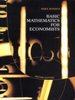
ThesevaluesindicatethatthegraphisaU-shape,asshowninFigure6.1.Thiscutsthe
horizontal axis twice and so there are two values of q for which y is zero, which means that
there are two solutions to the question. The precise values of these solutions, 2.5 and 40, can
be found by the other two methods explained in the following sections or by computation of
y for different values of q. (See spreadsheet solution method below.)
If we slightly change the problem in Example 6.1 we can see why there may not always
be a solution to a quadratic equation.
Example 6.2
Find out if there is an output level at which total revenue is 1,500 for the function
TR = 85q − 2q
2
© 1993, 2003 Mike Rosser
q
y
200
–700
10 20 30–10 40
y =2q
2
–85q + 200

550
50 60
Figure 6.1
Solution
The quadratic equation to be solved is
1,500 = 85q − 2q
2
which can be rewritten as
2q
2
− 85q + 1,500 = 0
If we now specify the new function
y = 2q
2
− 85q + 1,500
and calculate a few values, we can see that it falls and then rises again but never cuts the
qaxis,asFigure6.2shows.
When q = 0, then y = 1,500
When q = 10, then y = 850
When q = 20, then y = 600
When q = 25, then y = 625
There are therefore no solutions to this quadratic equation, i.e. there is no output at which
total revenue will be 1,500.
© 1993, 2003 Mike Rosser
y=2q
2
–85q+1,500
q
y
60203050–1040

1,500
600
10
Figure6.2
Althoughonewouldnevertrytoplotthewholegraphofaquadraticfunctionmanually,
onemayofcoursegetacomputerplot.Theaccuracyoftheansweryouobtainwilldepend
onthegraphicspackagethatyouuse.
PlottingquadraticfunctionswithExcel
AnExcelspreadsheetforcalculatingdifferentvaluesofthefunctionyinExample6.1above
canbeconstructedbyfollowingtheinstructionsinTable6.1.Ratherthanbuildinginformulae
thatarespecifictothisexample,thisspreadsheetisconstructedinaformatthatcanbeused
toplotanyfunctionintheformy=aq
2
+bq+concetheparametersa,bandcareentered
intherelevantcells.Therangeforqhasbeenchosentoensurethatitincludesthevalues
whenyiszero,whichiswhatweareinterestedinfinding.
IfyouconstructthisspreadsheetyoushouldgettheseriesofvaluesshowninTable6.2.
The q values which correspond to a y value of zero can now be read off, giving the solutions
2.5 and 40.
You may also use the Excel spreadsheet you have created to plot a graph of the function
y = 2q
2
−85q +200. Assuming that you have q and y in single columns, then you just use
the Chart Wizard command to obtain a plot with q measured on the X axis and y as variable
A on the vertical axis. (It you don’t know how to use this chart command, refer back to
Example4.17.)Tomakethechartclearertoread,enlargeitabitbydraggingthecorner.The
legend box for y can also be cut out to allow the chart area to be enlarged. This should give
youaplotsimilartoFigure6.3,whichclearlyshowshowthisfunctioncutsthehorizontal
axis twice.
© 1993, 2003 Mike Rosser