foundations of econometrics phần 5 ppsx

7.7 Testing for Serial Correlation 279
the alternative that ρ > 0. An investigator will reject the null hypothesis if
d < d
L
, fail to reject if d > d
U
, and come to no conclusion if d
L
< d < d
U
.
For example, for a test at the .05 level when n = 100 and k = 8, including the
constant term, the bounding critical values are d
L
= 1.528 and d
U
= 1.826.
Therefore, one would reject the null hypothesis if d < 1.528 and not reject it
if d > 1.826. Notice that, even for this not particularly small sample size, the
indeterminate region between 1.528 and 1.826 is quite large.
It should by now be evident that the Durbin-Watson statistic, despite its
popularity, is not very satisfactory. Using it with standard tables is relatively
cumbersome and often yields inconclusive results. Moreover, the standard
tables only allow us to perform one-tailed tests against the alternative that
ρ > 0. Since the alternative that ρ < 0 is often of interest as well, the inability
to perform a two-tailed test, or a one-tailed test against this alternative, using
standard tables is a serious limitation. Although exact P values for both one-
tailed and two-tailed tests, which depend on the X matrix, can be obtained
by using appropriate software, many computer programs do not offer this
capability. In addition, the DW statistic is not valid when the regressors
include lagged dependent variables, and it cannot easily be generalized to test

for higher-order processes. Happily, the development of simulation-based tests
has made the DW statistic obsolete.
Monte Carlo Tests for Serial Correlation
We discussed simulation-based tests, including Monte Carlo tests and boot-
strap tests, at some length in Section 4.6. The techniques discussed there can
readily be applied to the problem of testing for serial correlation in linear and
nonlinear regression models.
All the test statistics we have discussed, namely, t
GNR
, t
SR
, and d, are pivotal
under the null hypothesis that ρ = 0 when the assumptions of the classical
normal linear model are satisfied. This makes it possible to perform Monte
Carlo tests that are exact in finite samples. Pivotalness follows from two
properties shared by all these statistics. The first of these is that they depend
only on the residuals ˜u
t
obtained by estimation under the null hyp othesis.
The distribution of the residuals depends on the exogenous explanatory vari-
ables X, but these are given and the same for all DGPs in a classical normal
linear model. The distribution does not depend on the parameter vector β of
the regression function, because, if y = Xβ + u, then M
X
y = M
X
u what-
ever the value of the vector β.
The second property that all the statistics we have considered share is scale
invariance. By this, we mean that multiplying the dependent variable by

an arbitrary scalar λ leaves the statistic unchanged. In a linear regression
model, multiplying the dependent variable by λ causes the residuals to be
multiplied by λ. But the statistics defined in (7.51), (7.52), and (7.53) are
clearly unchanged if all the residuals are multiplied by the same constant, and
so these statistics are scale invariant. Since the residuals
˜
u are equal to M
X
u,
Copyright
c
 1999, Russell Davidson and James G. MacKinnon
280 Generalized Least Squares and Related Topics
it follows that multiplying σ by an arbitrary λ multiplies the residuals by λ.
Consequently, the distributions of the statistics are independent of σ
2
as well
as of β. This implies that, for the classical normal linear model, all three
statistics are pivotal.
We now outline how to perform Monte Carlo tests for serial correlation in the
context of the classical normal linear model. Let us call the test statistic we
are using τ and its realized value ˆτ. If we want to test for AR(1) errors, the
best choice for the statistic τ is the t statistic t
GNR
from the GNR (7.43), but
it could also be the DW statistic, the t statistic t
SR
from the simple regression
(7.46), or even ˜ρ itself. If we want to test for AR(p) errors, the best choice
for τ would be the F statistic from the GNR (7.45), but it could also be the

F statistic from a regression of ˜u
t
on ˜u
t−1
through ˜u
t−p
.
The first step, evidently, is to compute ˆτ. The next step is to generate B sets
of simulated residuals and use each of them to compute a simulated test
statistic, say τ
∗
j
, for j = 1, . . . , B. Because the parameters do not matter,
we can simply draw B vectors u
∗
j
from the N(0, I) distribution and regress
each of them on X to generate the simulated residuals M
X
u
∗
j
, which are then
used to compute τ
∗
j
. This can be done very inexpensively. The final step is to
calculate an estimated P value for whatever null hypothesis is of interest. For
example, for a two-tailed test of the null hypothesis that ρ = 0, the P value
would be the proportion of the τ

∗
j
that exceed ˆτ in absolute value:
ˆp
∗
(ˆτ) =
1
B
B

j=1
I

|τ
∗
j
| > |ˆτ|

. (7.54)
We would then reject the null hypothesis at level α if ˆp
∗
(ˆτ) < α. As we saw
in Section 4.6, such a test will be exact whenever B is chosen so that α(B + 1)
is an integer.
Bootstrap Tests for Serial Correlation
Whenever the regression function is nonlinear or contains lagged dependent
variables, or whenever the distribution of the error terms is unknown, none of
the standard test statistics for serial correlation will be pivotal. Nevertheless,
it is still possible to obtain very accurate inferences, even in quite small sam-
ples, by using bootstrap tests. The procedure is essentially the one described

in the previous subsection. We still generate B simulated test statistics and
use them to compute a P value according to (7.54) or its analog for a one-
tailed test. For best results, the test statistic used should be asymptotically
valid for the model that is being tested. In particular, we should avoid d and
t
SR
whenever there are lagged dependent variables.
It is extremely important to generate the bootstrap samples in such a way that
they are compatible with the model under test. Ways of generating bootstrap
samples for regression models were discussed in Section 4.6. If the mo del
Copyright
c
 1999, Russell Davidson and James G. MacKinnon
7.7 Testing for Serial Correlation 281
is nonlinear or includes lagged dependent variables, we need to generate y
∗
j
rather than just u
∗
j
. For this, we need estimates of the parameters of the
regression function. If the model includes lagged dependent variables, we
must generate the bootstrap samples recursively, as in (4.66). Unless we are
going to assume that the error terms are normally distributed, we should
draw the bootstrap error terms from the EDF of the residuals for the model
under test, after they have been appropriately rescaled. Recall that there is
more than one way to do this. The simplest approach is just to multiply each
residual by (n/(n − k))
1/2
, as in expression (4.68).

We strongly recommend the use of simulation-based tests for serial correla-
tion, rather than asymptotic tests. Monte Carlo tests are appropriate only
in the context of the classical normal linear model, but bootstrap tests are
appropriate under much weaker assumptions. It is generally a good idea to
test for b oth AR(1) errors and higher-order autoregressive errors, at least
fourth-order in the case of quarterly data, and at least twelfth-order in the
case of monthly data.
Heteroskedasticity-Robust Tests
The tests for serial correlation that we have discussed are based on the assump-
tion that the error terms are homoskedastic. When this crucial assumption is
violated, the asymptotic distributions of all the test statistics will differ from
whatever distributions they are supposed to follow asymptotically. However,
as we saw in Section 6.8, it is not difficult to modify GNR-based tests to make
them robust to heteroskedasticity of unknown form.
Suppose we wish to test the linear regression model (7.42), in which the error
terms are serially uncorrelated, against the alternative that the error terms
follow an AR(p) process. Under the assumption of homoskedasticity, we could
simply run the GNR (7.45) and use an asymptotic F test. If we let Z denote
an n × p matrix with typical element Z
ti
= ˜u
t−i
, where any missing lagged
residuals are replaced by zeros, this GNR can be written as
˜
u = Xb + Zc + residuals. (7.55)
The ordinary F test for c = 0 in (7.55) is not robust to heteroskedasticity, but
a heteroskedasticity-robust test can easily be computed using the procedure
described in Section 6.8. This procedure works as follows:
1. Create the matrices

˜
UX and
˜
UZ by multiplying the t
th
row of X and
the t
th
row of Z by ˜u
t
for all t.
2. Create the matrices
˜
U
−1
X and
˜
U
−1
Z by dividing the t
th
row of X and
the t
th
row of Z by ˜u
t
for all t.
3. Regress each of the columns of
˜
U

−1
X and
˜
U
−1
Z on
˜
UX and
˜
UZ jointly.
Save the resulting matrices of fitted values and call them
¯
X and
¯
Z,
respectively.
Copyright
c
 1999, Russell Davidson and James G. MacKinnon
282 Generalized Least Squares and Related Topics
4. Regress ι, a vector of 1s, on
¯
X. Retain the sum of squared residuals from
this regression, and call it RSSR. Then regress ι on
¯
X and
¯
Z jointly,
retain the sum of squared residuals, and call it USSR.
5. Compute the test statistic RSSR − USSR, which will be asymptotically

distributed as χ
2
(p) under the null hypothesis.
Although this heteroskedasticity-robust test is asymptotically valid, it will
not be exact in finite samples. In principle, it should be possible to obtain
more reliable results by using bootstrap P values instead of asymptotic ones.
However, none of the metho ds of generating bootstrap samples for regression
models that we have discussed so far (see Section 4.6) is appropriate for a
model with heteroskedastic error terms. Several methods exist, but they are
beyond the scope of this book, and there currently exists no method that we
can recommend with complete confidence; see Davison and Hinkley (1997)
and Horowitz (2001).
Other Tests Based on OLS Residuals
The tests for serial correlation that we have discussed in this section are by
no means the only scale-invariant tests based on least squares residuals that
are regularly encountered in econometrics. Many tests for heteroskedasticity,
skewness, kurtosis, and other deviations from the NID assumption also have
these properties. For example, consider tests for heteroskedasticity based
on regression (7.28). Nothing in that regression depends on y except for the
squared residuals that constitute the regressand. Further, it is clear that both
the F statistic for the hypothesis that b
γ
= 0 and n times the centered R
2
are
scale invariant. Therefore, for a classical normal linear model with X and Z
fixed, these statistics are pivotal. Consequently, Monte Carlo tests based on
them, in which we draw the error terms from the N(0, 1) distribution, are
exact in finite samples.
When the normality assumption is not appropriate, we have two options. If

some other distribution that is known up to a scale parameter is thought to be
appropriate, we can draw the error terms from it instead of from the N(0, 1)
distribution. If the assumed distribution really is the true one, we obtain
an exact test. Alternatively, we can perform a bootstrap test in which the
error terms are obtained by resampling the rescaled residuals. This is also
appropriate when there are lagged dependent variables among the regressors.
The bootstrap test will not be exact, but it should still perform well in finite
samples no matter how the error terms actually happen to be distributed.
7.8 Estimating Models with Autoregressive Errors
If we decide that the error terms of a regression model are serially correlated,
either on the basis of theoretical considerations or as a result of specification
Copyright
c
 1999, Russell Davidson and James G. MacKinnon
7.8 Estimating Models with Autoregressive Errors 283
testing, and we are confident that the regression function itself is not misspec-
ified, the next step is to estimate a modified model which takes account of
the serial correlation. The simplest such model is (7.40), which is the original
regression model modified by having the error terms follow an AR(1) process.
For ease of reference, we rewrite (7.40) here:
y
t
= X
t
β + u
t
, u
t
= ρu
t−1

+ ε
t
, ε
t
∼ IID(0, σ
2
ε
). (7.56)
In many cases, as we will discuss in the next section, the best approach may
actually be to specify a more complicated, dynamic, model for which the
error terms are not serially correlated. In this section, however, we ignore this
important issue and simply discuss how to estimate the model (7.56) under
various assumptions.
Estimation by Feasible GLS
We have seen that, if the u
t
follow a stationary AR(1) process, that is, if
|ρ| < 1 and Var(u
1
) = σ
2
u
= σ
2
ε
/(1 − ρ
2
), then the covariance matrix of
the entire vector u is the n × n matrix Ω(ρ) given in (7.32). In order to
compute GLS estimates, we need to find a matrix Ψ with the property that

Ψ Ψ

= Ω
−1
. This property will be satisfied whenever the covariance matrix
of Ψ

u is proportional to the identity matrix, which it will be if we choose Ψ
in such a way that Ψ

u = ε.
For t = 2, . . . , n, we know from (7.29) that
ε
t
= u
t
− ρu
t−1
, (7.57)
and this allows us to construct the rows of Ψ

except for the first row. The
t
th
row must have 1 in the t
th
position, −ρ in the (t − 1)
st
position, and 0s
everywhere else.

For the first row of Ψ

, however, we need to be a little more careful. Under
the hypothesis of stationarity of u, the variance of u
1
is σ
2
u
. Further, since
the ε
t
are innovations, u
1
is uncorrelated with the ε
t
for t = 2, . . . , n. Thus,
if we define ε
1
by the formula
ε
1
= (σ
ε
/σ
u
)u
1
= (1 − ρ
2
)

1/2
u
1
, (7.58)
it can be seen that the n vector ε, with the first component ε
1
defined
by (7.58) and the remaining components ε
t
defined by (7.57), has a covar-
iance matrix equal to σ
2
ε
I.
Putting together (7.57) and (7.58), we conclude that Ψ

should be defined
as an n × n matrix with all diagonal elements equal to 1 except for the first,
which is equal to (1 − ρ
2
)
1/2
, and all other elements equal to 0 except for
Copyright
c
 1999, Russell Davidson and James G. MacKinnon
284 Generalized Least Squares and Related Topics
the ones on the diagonal immediately below the principal diagonal, which are
equal to −ρ. In terms of Ψ rather than of Ψ


, we have:
Ψ (ρ) =







(1 − ρ
2
)
1/2
−ρ 0 · · · 0 0
0 1 −ρ · · · 0 0
.
.
.
.
.
.
.
.
.
.
.
.
.
.
.

0 0 0 · · · 1 −ρ
0 0 0 · · · 0 1







, (7.59)
where the notation Ψ(ρ) emphasizes that the matrix depends on the usually
unknown parameter ρ. The calculations needed to show that the matrix Ψ Ψ

is proportional to the inverse of Ω, as given by (7.32), are outlined in Exercises
7.9 and 7.10.
It is essential that the AR(1) parameter ρ either be known or be consistently
estimable. If we know ρ, we can obtain GLS estimates. If we do not know it
but can estimate it consistently, we can obtain feasible GLS estimates. For the
case in which the explanatory variables are all exogenous, the simplest way
to estimate ρ consistently is to use the estimator ˜ρ from regression (7.46),
defined in (7.47). Whatever estimate of ρ is used must satisfy the stationarity
condition that |ρ| < 1, without which the process would not be stationary, and
the transformation for the first observation would involve taking the square
root of a negative number. Unfortunately, the estimator ˜ρ is not guaranteed
to satisfy the stationarity condition, although, in practice, it is very likely to
do so when the model is correctly specified, even if the true value of ρ is quite
large in absolute value.
Whether ρ is known or estimated, the next step in GLS estimation is to form
the vector Ψ


y and the matrix Ψ

X. It is easy to do this without having to
store the n × n matrix Ψ in computer memory. The first element of Ψ

y is
(1 − ρ
2
)
1/2
y
1
, and the remaining elements have the form y
t
− ρy
t−1
. Each
column of Ψ

X has precisely the same form as Ψ

y and can be calculated in
precisely the same way.
The final step is to run an OLS regression of Ψ

y on Ψ

X. This regression
yields the (feasible) GLS estimates
ˆ

β
GLS
= (X

Ψ Ψ

X)
−1
X

Ψ Ψ

y (7.60)
along with the estimated covariance matrix

Var(
ˆ
β
GLS
) = s
2
(X

Ψ Ψ

X)
−1
, (7.61)
where s
2

is the usual OLS estimate of the variance of the error terms. Of
course, the estimator (7.60) is formally identical to (7.04), since (7.60) is valid
for any Ψ matrix.
Copyright
c
 1999, Russell Davidson and James G. MacKinnon
7.8 Estimating Models with Autoregressive Errors 285
Estimation by Nonlinear Least Squares
If we ignore the first observation, then (7.56), the linear regression model
with AR(1) errors, can be written as the nonlinear regression model (7.41).
Since the model (7.41) is written in such a way that the error terms are inno-
vations, NLS estimation is consistent whether the explanatory variables are
exogenous or merely predetermined. NLS estimates can be obtained by any
standard nonlinear minimization algorithm of the type that was discussed
in Section 6.4, where the function to be minimized is SSR(β, ρ), the sum of
squared residuals for observations 2 through n. Such procedures generally
work well, and they can also be used for models with higher-order autoregres-
sive errors; see Exercise 7.17. However, some care must be taken to ensure
that the algorithm does not terminate at a local minimum which is not also
the global minimum. There is a serious risk of this, especially for models with
lagged dependent variables among the regressors.
2
Whether or not there are lagged dependent variables in X
t
, a valid estimated
covariance matrix can always be obtained by running the GNR (6.67), which
corresponds to the model (7.41), with all variables evaluated at the NLS
estimates
ˆ
β and ˆρ. This GNR is

y
t
− ˆρy
t−1
− X
t
ˆ
β + ˆρX
t−1
ˆ
β
= (X
t
− ˆρX
t−1
)b + b
ρ
(y
t−1
− X
t−1
ˆ
β) + residual.
(7.62)
Since the OLS estimates of b and b
ρ
will be equal to zero, the sum of squared
residuals from regression (7.62) is simply SSR(
ˆ
β, ˆρ). Therefore, the estimated

covariance matrix

Var(
ˆ
β, ˆρ) is
SSR(
ˆ
β, ˆρ)
n − k − 2

(X − ˆρX
1
)

(X − ˆρX
1
) (X − ˆρX
1
)

ˆ
u
1
ˆ
u
1

(X − ˆρX
1
)

ˆ
u
1

ˆ
u
1

−1
, (7.63)
where the n×k matrix X
1
has typical row X
t−1
, and the vector
ˆ
u
1
has typical
element y
t−1
− X
t−1
ˆ
β. This is the estimated covariance matrix that a good
nonlinear regression package should print. The first factor in (7.63) is just
the NLS estimate of σ
2
ε
. The SSR is divided by n − k − 2 because there are

k + 1 parameters in the regression function, one of which is ρ, and we estimate
using only n − 1 observations.
It is instructive to compute the limit in probability of the matrix (7.63) when
n → ∞ for the case in which all the explanatory variables in X
t
are exogenous.
The parameters are all estimated consistently by NLS, and so the estimates
converge to the true parameter values β
0
, ρ
0
, and σ
2
ε
as n → ∞. In computing
the limit of the denominator of the simple estimator ˜ρ given by (7.47), we saw
that n
−1
ˆ
u
1

ˆ
u
1
tends to σ
2
ε
/(1 − ρ
2

0
). The limit of n
−1
(X − ˆρX
1
)

ˆ
u
1
is the
2
See Dufour, Gaudry, and Liem (1980) and Betancourt and Kelejian (1981).
Copyright
c
 1999, Russell Davidson and James G. MacKinnon
286 Generalized Least Squares and Related Topics
same as that of n
−1
(X −ρ
0
X
1
)

ˆ
u
1
by the consistency of ˆρ. In addition, given
the exogeneity of X, and thus also of X

1
, it follows at once from the law of
large numbers that n
−1
(X − ρ
0
X
1
)

ˆ
u
1
tends to zero. Thus, in this special
case, the asymptotic covariance matrix of n
1/2
(
ˆ
β − β
0
) and n
1/2
(ˆρ − ρ
0
) is
σ
2
ε

plim

1
−
n
(X − ρ
0
X
1
)

(X − ρ
0
X
1
) 0
0

σ
2
ε
/(1 − ρ
2
0
)

−1
. (7.64)
Because the two off-diagonal blocks are zero, this matrix is said to be block-
diagonal. As can be verified immediately, the inverse of such a matrix is itself a
block-diagonal matrix, of which each block is the inverse of the corresponding
block of the original matrix. Thus the asymptotic covariance matrix (7.64) is

the limit as n → ∞ of

nσ
2
ε

(X − ρ
0
X
1
)

(X − ρ
0
X
1
)

−1
0
0

1 − ρ
2
0

. (7.65)
The block-diagonality of (7.65), which holds only if everything in X
t
is exo-

genous, implies that the covariance matrix of
ˆ
β can be estimated using the
GNR (7.62) without the regressor corresponding to ρ. The estimated covar-
iance matrix will just be (7.63) without its last row and column. It is easy to
see that n times this matrix tends to the top left block of (7.65) as n → ∞.
The lower right-hand element of the matrix (7.65) tells us that, when all the
regressors are exogenous, the asymptotic variance of n
1/2
(ˆρ − ρ
0
) is 1 − ρ
2
0
.
A sensible estimate of the variance is therefore

Var(ˆρ) = n
−1
(1 − ˆρ
2
). It may
seem surprising that the variance of ˆρ does not depend on σ
2
ε
. However, we saw
earlier that, with exogenous regressors, the consistent estimator ˜ρ of (7.47) is
scale invariant. The same is true, asymptotically, of the NLS estimator ˆρ, and
so its asymptotic variance is independent of σ
2

ε
.
Comparison of GLS and NLS
The most obvious difference between estimation by GLS and estimation by
NLS is the treatment of the first observation: GLS takes it into account, and
NLS does not. This difference reflects the fact that the two procedures are
estimating slightly different models. With NLS, all that is required is the
stationarity condition that |ρ| < 1. With GLS, on the other hand, the error
process must actually be stationary. Recall that the stationarity condition is
necessary but not sufficient for stationarity of the process. A sufficient con-
dition requires, in addition, that Var(u
1
) = σ
2
u
= σ
2
ε
/(1 − ρ
2
), the stationary
value of the variance. Thus, if we suspect that Var(u
1
) = σ
2
u
, GLS estimation
is not appropriate, because the matrix (7.32) is not the covariance matrix of
the error terms.
The second major difference between estimation by GLS and estimation by

NLS is that the former method estimates β conditional on ρ, while the latter
Copyright
c
 1999, Russell Davidson and James G. MacKinnon
7.8 Estimating Models with Autoregressive Errors 287
method estimates β and ρ jointly. Except in the unlikely case in which the
value of ρ is known, the first step in GLS is to estimate ρ consistently. If
the explanatory variables in the matrix X are all exogenous, there are several
procedures that will deliver a consistent estimate of ρ. The weak point is
that the estimate is not unique, and in general it is not optimal. One possible
solution to this difficulty is to iterate the feasible GLS procedure, as suggested
at the end of Section 7.4, and we will consider this solution below.
A more fundamental weakness of GLS arises whenever one or more of the
explanatory variables are lagged dependent variables, or, more generally, pre-
determined but not exogenous variables. Even with a consistent estimator
of ρ, one of the conditions for the applicability of feasible GLS, condition
(7.23), does not hold when any elements of X
t
are not exogenous. It is not
simple to see directly just why this is so, but, in the next paragraph, we will
obtain indirect evidence by showing that feasible GLS gives an invalid estima-
tor of the covariance matrix. Fortunately, there is not much temptation to use
GLS if the non-exogenous explanatory variables are lagged variables, because
lagged variables are not observed for the first observation. In all events, the
conclusion is simple: We should avoid GLS if the explanatory variables are
not all exogenous.
The GLS covariance matrix estimator is (7.61), which is obtained by regressing
Ψ

(ˆρ)y on Ψ


(ˆρ)X for some consistent estimate ˆρ. Since Ψ

(ρ)u = ε by
construction, s
2
is an estimator of σ
2
ε
. Moreover, the first observation has no
impact asymptotically. Therefore, the limit as n → ∞ of n times (7.61) is the
matrix
σ
2
ε
plim
n→∞

1
−
n
(X − ρX
1
)

(X − ρX
1
)

−1

. (7.66)
In contrast, the NLS covariance matrix estimator is (7.63). With exogenous
regressors, n times (7.63) tends to the same limit as (7.65), of which the top
left block is just (7.66). But when the regressors are not all exogenous, the
argument that the off-diagonal blocks of n times (7.63) tend to zero no longer
works, and, in fact, the limits of these blocks are in general nonzero. When a
matrix that is not block-diagonal is inverted, the top left block of the inverse
is not the same as the inverse of the top left blo ck of the original matrix;
see Exercise 7.11. In fact, as readers are asked to show in Exercise 7.12, the
top left block of the inverse is greater by a positive semidefinite matrix than
the inverse of the top left block. Consequently, the GLS covariance matrix
estimator underestimates the true covariance matrix asymptotically.
NLS has only one major weak point, which is that it does not take account of
the first observation. Of course, this is really an advantage if the error process
satisfies the stationarity condition without actually being stationary, or if
some of the explanatory variables are not exogenous. But with a stationary
error process and exogenous regressors, we wish to retain the information in
the first observation, because it appears that retaining the first observation
can sometimes lead to a noticeable efficiency gain in finite samples. The
Copyright
c
 1999, Russell Davidson and James G. MacKinnon
288 Generalized Least Squares and Related Topics
reason is that the transformation for observation 1 is quite different from the
transformation for all the other observations. In consequence, the transformed
first observation may well be a high leverage point; see Section 2.6. This
is particularly likely to happen if one or more of the regressors is strongly
trending. If so, dropping the first observation can mean throwing away a lot
of information. See Davidson and MacKinnon (1993, Section 10.6) for a much
fuller discussion and references.

Efficient Estimation by GLS or NLS
When the error process is stationary and all the regressors are exogenous, it
is possible to obtain an estimator with the best features of GLS and NLS by
modifying NLS so that it makes use of the information in the first observation
and therefore yields an efficient estimator. The first-order conditions (7.07)
for GLS estimation of the model (7.56) can be written as
X

Ψ Ψ

(y − Xβ) = 0.
Using (7.59) for Ψ , we see that these conditions are
n

t=2
(X
t
− ρX
t−1
)


y
t
− X
t
β − ρ(y
t−1
− X
t−1

β)

+ (1 − ρ
2
)X
1

(y
1
− X
1
β) = 0.
(7.67)
With NLS estimation, the first-order conditions that define the NLS estimator
are the conditions that the regressors in the GNR (7.62) should be orthogonal
to the regressand:
n

t=2
(X
t
− ρX
t−1
)


y
t
− X
t

β − ρ(y
t−1
− X
t−1
β)

= 0, and
n

t=2
(y
t−1
− X
t−1
β)

y
t
− X
t
β − ρ(y
t−1
− X
t−1
β)

= 0.
(7.68)
For given β, the second of the NLS conditions can be solved for ρ. If we write
u(β) = y − Xβ, and u

1
(β) = Lu(β), where L is the matrix lag operator
defined in (7.49), we see that
ρ(β) =
u

(β)u
1
(β)
u
1

(β)u
1
(β)
. (7.69)
This formula is similar to the estimator (7.47), except that β may take on
any value instead of just
˜
β.
In Section 7.4, we mentioned the possibility of using an iterated feasible GLS
procedure. We can now see precisely how such a procedure would work for
this model. In the first step, we obtain the OLS parameter vector
˜
β. In the
Copyright
c
 1999, Russell Davidson and James G. MacKinnon
7.8 Estimating Models with Autoregressive Errors 289
second step, the formula (7.69) is evaluated at β =

˜
β to obtain ˜ρ, a consistent
estimate of ρ. In the third step, we use (7.60) to obtain the feasible GLS
estimate
ˆ
β
F
, thus solving the first-order conditions (7.67). At this point, we
go back to the second step and insert
ˆ
β
F
into (7.69) for an updated estimate
of ρ, which we subsequently use in (7.60) for the next estimate of β. The
iterative procedure may then be continued until convergence, assuming that
it does converge. If so, then the final estimates, which we will call
ˆ
β and ˆρ,
must satisfy the two equations
n

t=2
(X
t
− ˆρX
t−1
)


y

t
− X
t
ˆ
β − ˆρ(y
t−1
− X
t−1
ˆ
β)

+ (1 − ˆρ
2
)X
1

(y
1
− X
1
ˆ
β) = 0, and
n

t=2
(y
t−1
− X
t−1
ˆ

β)

y
t
− X
t
ˆ
β − ˆρ(y
t−1
− X
t−1
ˆ
β)

= 0.
(7.70)
These conditions are identical to conditions (7.68), except for the term in the
first condition coming from the first observation. Thus we see that iterated
feasible GLS, without the first observation, is identical to NLS. If the first
observation is retained, then iterated feasible GLS improves on NLS by taking
account of the first observation.
We can also modify NLS to take account of the first observation. To do this,
we extend the GNR (6.67), which is given by (7.62) when evaluated at
ˆ
β
and ˆρ, by giving it a first observation. For this observation, the regressand
is (1 − ρ
2
)
1/2

(y
1
− X
1
β), the regressors corresponding to β are given by the
row vector (1 − ρ
2
)
1/2
X
1
, and the regressor corresponding to ρ is zero. The
conditions that the extended regressand should be orthogonal to the extended
regressors are exactly the conditions (7.70).
Two asymptotically equivalent procedures can be based on this extended
GNR. Both begin by obtaining the NLS estimates of β and ρ without the
first observation and evaluating the extended GNR at those preliminary NLS
estimates. The OLS estimates from the extended GNR can be thought of as
a vector of corrections to the initial estimates. For the first procedure, the
final estimator is a one-step estimator, defined as in (6.59) by adding the cor-
rections to the preliminary estimates. For the second procedure, this process
is iterated. The variables of the extended GNR are evaluated at the one-step
estimates, another set of corrections is obtained, these are added to the pre-
vious estimates, and iteration continues until the corrections are negligible. If
this happens, the iterated estimates once more satisfy the conditions (7.70),
and so they are equal to the iterated GLS estimates.
Although the iterated feasible GLS estimator generally performs well, it does
have one weakness: There is no way to ensure that |ˆρ| < 1. In the unlikely
but not impossible event that |ˆρ| ≥ 1, the estimated covariance matrix (7.61)
will not be valid, the second term in (7.67) will be negative, and the first

observation will therefore tend to have a perverse effect on the estimates of β.
Copyright
c
 1999, Russell Davidson and James G. MacKinnon
290 Generalized Least Squares and Related Topics
In Chapter 10, we will see that maximum likelihood estimation shares the
good properties of iterated feasible GLS while also ensuring that the estimate
of ρ satisfies the stationarity condition.
The iterated feasible GLS procedure considered above has much in common
with a very old, but still widely-used, algorithm for estimating models with
stationary AR(1) errors. This algorithm, which is called iterated Cochrane-
Orcutt, was originally proposed in a classic paper by Cochrane and Orcutt
(1949). It works in exactly the same way as iterated feasible GLS, except that
it omits the first observation. The properties of this algorithm are explored
in Exercises 7.18-19.
7.9 Specification Testing and Serial Correlation
Models estimated using time-series data frequently appear to have error terms
which are serially correlated. However, as we will see, many types of misspec-
ification can create the appearance of serial correlation. Therefore, finding
evidence of serial correlation does not mean that it is necessarily appropriate
to model the error terms as following some sort of autoregressive or moving
average process. If the regression function of the original model is misspecified
in any way, then a model like (7.41), which has been modified to incorporate
AR(1) errors, will probably also be misspecified. It is therefore extremely
important to test the specification of any regression model that has been
“corrected” for serial correlation.
The Appearance of Serial Correlation
There are several types of misspecification of the regression function that can
incorrectly create the appearance of serial correlation. For instance, it may be
that the true regression function is nonlinear in one or more of the regressors

while the estimated one is linear. In that case, depending on how the data
are ordered, the residuals from a linear regression model may well appear to
be serially correlated. All that is needed is for the independent variables on
which the dependent variable depends nonlinearly to be correlated with time.
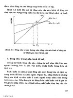
As a concrete example, consider Figure 7.1, which shows 200 hypothetical
observations on a regressor x and a regressand y, together with an OLS re-
gression line and the fitted values from the true, nonlinear model. For the
linear model, the residuals are always negative for the smallest and largest
values of x, and they tend to be positive for the intermediate values. As a
consequence, they appear to be serially correlated: If the observations are
ordered according to the value of x, the estimate ˜ρ obtained by regressing the
OLS residuals on themselves lagged once is 0.298, and the t statistic for ρ = 0
is 4.462. Thus, if the data are ordered in this way, there appears to be strong
evidence of serial correlation. But this evidence is misleading. Either plotting
the residuals against x or including x
2
as an additional regressor will quickly
reveal the true nature of the misspecification.
Copyright
c
 1999, Russell Davidson and James G. MacKinnon
7.9 Specification Testing and Serial Correlation 291
.
.
.
.
.
.
.
.

.
.
.
.
.
.
.
.
.
.
.
.
.
.
.
.
.
.
.
.
.
.
.
.
.
.
.
.
.
.

.
.
.
.
.
.
.
.
.
.
.
.
.
.
.
.
.
.
.
.
.
.
.
.
.
.
.
.
.
.

.
.
.
.
.
.
.
.
.
.
.
.
.
.
.
.
.
.
.
.
.
.
.
.
.
.
.
.
.
.

.
.
.
.
.
.
.
.
.
.
.
.
.
.
.
.
.
.
.
.
.
.
.
.
.
.
.
.
.
.

.
.
.
.
.
.
.
.
.
.
.
.
.
.
.
.
.
.
.
.
.
.
.
.
.
.
.
.
.
.

.
.
.
.
.
.
.
.
.
.
.
.
.
.
.
.
.
.
.
.
.
.
.
.
.
.
.
.
.
.

.
.
.
.
.
.
.
.
.
.
.
.
.
.
.
.
.
.
.
.
.
.
.
.
.
.
.
.
.
.

.
.
.
.
.
.
.
.
.
.
.
.
.
.
.
.
.
.
.
.
.
.
.
.
.
.
.
.
.
.

.
.
.
.
.
.
.
.
.
.
.
.
.
.
.
.
.
.
.
.
.
.
.
.
.
.
.
.
.
.

.
.
.
.
.
.
.
.
.
.
.
.
.
.
.
.
.
.
.
.
.
.
.
.
.
.
.
.
.
.

.
.
.
.
.
.
.
.
.
.
.
.
.
.
.
.
.
.
.
.
.
.
.
.
.
.
.
.
.
.

.
.
.
.
.
.
.
.
.
.
.
.
.
.
.
.
.
.
.
.
.
.
.
.
.
.
.
.
.
.

.
.
.
.
.
.
.
.
.
.
.
.
.
.
.
.
.
.
.
.
.
.
.
.
.
.
.
.
.
.

.
.
.
.
.
.
.
.
.
.
.
.
.
.
.
.
.
.
.
.
.
.
.
.
.
.
.
.
.
.

.
.
.
.
.
.
.
.
.
.
.
.
.
.
.
.
.
.
.
.
.
.
.
.
.
.
.
.
.
.

.
.
.
.
.
.
.
.
.
.
.
.
.
.
.
.
.
.
.
.
.
.
.
.
.
.
.
.
.
.

.
.
.
.
.
.
.
.
.
.
.
.
.
.
.
.
.
.
.
.
.
.
.
.
.
.
.
.
.
.

.
.
.
.
.
.
.
.
.
.
.
.
.
.
.
.
.
.
.
.
.
.
.
.
.
.
.
.
.
.

.
.
.
.
.
.
.
.
.
.
.
.
.
.
.
.
.
.
.
.
.
.
.
.
.
.
.
.
.
.

.
.
.
.
.
.
.
.
.
.
.
.
.
.
.
.
.
.
.
.
.
.
.
.
.
.
.
.
.
.

.
.
.
.
.
.
.
.
.
.
.
.
.
.
.
.
.
.
.
.
.
.
.
.
.
.
.
.
.
.

.
.
.
.
.
.
.
.
.
.
.
.
.
.
.
.
.
.
.
.
.
.
.
.
.
.
.
.
.
.

.
.
.
.
.
.
.
.
.
.
.
.
.
.
.
.
.
.
.
.
.
.
.
.
.
.
.
.
.
.

.
.
.
.
.
.
.
.
.
.
.
.
.
.
.
.
.
.
.
.
.
.
.
.
.
.
.
.
.
.

.
.
.
.
.
.
.
.
.
.
.
.
.
.
.
.
.
.
.
.
.
.
.
.
.
.
.
.
.
.

.
.
.
.
.
.
.
.
.
.
.
.
.
.
.
.
.
.
.
.
.
.
.
.
.
.
.
.
.
.

.
.
.
.
.
.
.
.
.
.
.
.
.
.
.
.
.
.
.
.
.
.
.
.
.
.
.
.
.
.

.
.
.
.
.
.
.
.
.
.
.
.
.
.
.
.
.
.
.
.
.
.
.
.
.
.
.
.
.
.

.
.
.
.
.
.
.
.
.
.
.
.
.
.
.
.
.
.
.
.
.
.
.
.
.
.
.
.
.
.

.
.
.
.
.
.
.
.
.
.
.
.
.
.
.
.
.
.
.
.
.
.
.
.
.
.
.
.
.
.

.
.
.
.
.
.
.
.
.
.
.
.
.
.
.
.
.
.
.
.
.
.
.
.
.
.
.
.
.
.

.
.
.
.
.
.
.
.
.
.
.
.
.
.
.
.
.
.
.
.
.
.
.
.
.
.
.
.
.
.

.
.
.
.
.
.
.
.
.
.
.
.
.
.
.
.
.
.
.
.
.
.
.
.
.
.
.
.
.
.

.
.
.
.
.
.
.
.
.
.
.
.
.
.
.
.
.
.
.
.
.
.
.
.
.
.
.
.
.
.

.
.
.
.
.
.
.
.
.
.
.
.
.
.
.
.
.
.
.
.
.
.
.
.
.
.
.
.
.
.

.
.
.
.
.
.
.
.
.
.
.
.
.
.
.
.
.
.
.
.
.
.
.
.
.
.
.
.
.
.

.
.
.
.
.
.
.
.
.
.
.
.
.
.
.
.
.
.
.
.
.
.
.
.
.
.
.
.
.
.

.
.
.
.
.
.
.
.
.
.
.
.
.
.
.
.
.
.
.
.
.
.
.
.
.
.
.
.
.
.

.
.
.
.
.
.
.
.
.
.
.
.
.
.
.
.
.
.
.
.
.
.
.
.
.
.
.
.
.
.

.
.
.
.
.
.
.
.
.
.
.
.
.
.
.
.
.
.
.
.
.
.
.
.
.
.
.
.
.
.

.
.
.
.
.
.
.
.
.
.
.
.
.
.
.
.
.
.
.
.

Regression line for linear model
.
.
.
.
.
.
.
.

.
.
.
.
.
.
.
.
.
.
.
.
.
.
.
.
.
.
.
.
.
.
.
.
.
.
.
.
.
.

.
.
.
.
.
.
.
.
.
.
.
.
.
.
.
.
.
.
.
.
.
.
.
.
.
.
.
.
.
.

.
.
.
.
.
.
.
.
.
.
.
.
.
.
.
.
.
.
.
.
.
.
.
.
.
.
.
.
.
.

.
.
.
.
.
.
.
.
.
.
.
.
.
.
.
.
.
.
.
.
.
.
.
.
.
.
.
.
.
.

.
.
.
.
.
.
.
.
.

.
.
.
.
.
.
.
.
.
.
.
.
.
.
.
.
.
.
.
.

.
.
.
.
.
.

Fitted values for true model
x
y
Figure 7.1 The appearance of serial correlation
The true regression function in this example contains a term in x
2
. Since
the linear model omits this term, it is underspecified, in the sense discussed
in Section 3.7. Any sort of underspecification has the potential to create
the appearance of serial correlation if the incorrectly omitted variables are
themselves serially correlated. Therefore, whenever we find evidence of serial
correlation, our first reaction should be to think carefully about the specifica-
tion of the regression function. Perhaps one or more additional independent
variables should be included among the regressors. Perhaps powers, cross-
products, or lags of some of the existing independent variables need to be
included. Or perhaps the regression function should be made dynamic by
including one or more lags of the dependent variable.
Common Factor Restrictions
It is very common for linear regression models to suffer from dynamic mis-
specification. The simplest example is failing to include a lagged dependent
variable among the regressors. More generally, dynamic misspecification oc-
curs whenever the regression function incorrectly omits lags of the dependent
variable or of one or more independent variables. A somewhat mechanical,

but often very effective, way to detect dynamic misspecification in models
with autoregressive errors is to test the common factor restrictions that are
implicit in such models. The idea of testing these restrictions was initially pro-
posed by Sargan (1964) and further developed by Hendry and Mizon (1978),
Mizon and Hendry (1980), Sargan (1980), and others. See Hendry (1995) for
a detailed treatment of dynamic specification in linear regression models.
Copyright
c
 1999, Russell Davidson and James G. MacKinnon
292 Generalized Least Squares and Related Topics
The easiest way to understand what common factor restrictions are and how
they got their name is to consider a linear regression model with errors that
apparently follow an AR(1) process. In this case, there are really three nested
models. The first of these is the original linear regression model with error
terms that are assumed to be serially independent:
H
0
: y
t
= X
t
β + u
t
, u
t
∼ IID(0, σ
2
). (7.71)
The second is the nonlinear model (7.41) that is obtained when the error
terms in (7.71) follow the AR(1) process (7.29). Although we have already

discussed this model extensively, we rewrite it here for convenience:
H
1
: y
t
= ρy
t−1
+ X
t
β − ρX
t−1
β + ε
t
, ε
t
∼ IID(0, σ
2
ε
). (7.72)
The third is the linear model that can be obtained by relaxing the nonlinear
restrictions which are implicit in (7.72). This model is
H
2
: y
t
= ρy
t−1
+ X
t
β + X

t−1
γ + ε
t
, ε
t
∼ IID(0, σ
2
ε
), (7.73)
where γ, like β, is a k vector. When all three of these models are estimated
over the same sample period, the original model, H
0
, is a special case of the
nonlinear model H
1
, which in turn is a special case of the unrestricted linear
model H
2
. Of course, in order to estimate H
1
and H
2
, we need to drop the
first observation.
The nonlinear model H
1
imposes on H
2
the restrictions that γ = −ρβ. The
reason for calling these restrictions “common factor” restrictions can easily be

seen if we rewrite both models using lag operator notation (see Section 7.6).
When we do this, H
1
becomes
(1 − ρL)y
t
= (1 − ρL)X
t
β + ε
t
, (7.74)
and H
2
becomes
(1 − ρL)y
t
= X
t
β + LX
t
γ + ε
t
. (7.75)
It is evident that in (7.74), but not in (7.75), the common factor 1 − ρL
appears on both sides of the equation. This is where the term “common
factor restrictions” comes from.
How Many Common Factor Restrictions Are There?
There is one feature of common factor restrictions that can be tricky: It is
often not obvious just how many restrictions there are. For the case of testing
H

1
against H
2
, there appear to be k restrictions. The null hypothesis, H
1
,
has k + 1 parameters (the k vector β and the scalar ρ), and the alternative
hypothesis, H
2
, seems to have 2k + 1 parameters (the k vectors β and γ,
and the scalar ρ). Therefore, the number of restrictions appears to be the
difference between 2k + 1 and k + 1, which is k. In fact, however, the number
Copyright
c
 1999, Russell Davidson and James G. MacKinnon
7.9 Specification Testing and Serial Correlation 293
of restrictions will almost always be less than k, because, except in rare cases,
the number of identifiable parameters in H
2
will be less than 2k + 1. We now
show why this is the case.
Let us consider a simple example. Suppose the regression function for the
original model H
0
is
β
1
+ β
2
z

t
+ β
3
t + β
4
z
t−1
+ β
5
y
t−1
, (7.76)
where z
t
is the t
th
observation on some independent variable, and t is the t
th
observation on a linear time trend. The regression function for the unrestricted
model H
2
that corresponds to (7.76) is
β
1
+ β
2
z
t
+ β
3

t + β
4
z
t−1
+ β
5
y
t−1
+ ρy
t−1
+ γ
1
+ γ
2
z
t−1
+ γ
3
(t − 1) + γ
4
z
t−2
+ γ
5
y
t−2
.
(7.77)
At first glance, this regression function appears to have 11 parameters. How-
ever, it really has only 7, because 4 of them are unidentifiable. We cannot

estimate both β
1
and γ
1
, because there cannot be two constant terms. Like-
wise, we cannot estimate both β
4
and γ
2
, because there cannot be two coef-
ficients of z
t−1
, and we cannot estimate both β
5
and ρ, because there cannot
be two coefficients of y
t−1
. We also cannot estimate γ
3
along with β
3
and
the constant, because t, t − 1, and the constant term are perfectly collinear,
since t − (t − 1) = 1. The version of H
2
that can actually be estimated has
regression function
δ
1
+ β

2
z
t
+ δ
2
t + δ
3
z
t−1
+ δ
4
y
t−1
+ γ
4
z
t−2
+ γ
5
y
t−2
, (7.78)
where
δ
1
= β
1
+ γ
1
− γ

3
, δ
2
= β
3
+ γ
3
, δ
3
= β
4
+ γ
2
, and δ
4
= ρ + β
5
.
We see that (7.78) has only 7 identifiable parameters: β
2
, γ
4
, γ
5
, δ
1
, δ
2
,
δ

3
, and δ
4
, instead of the 11 parameters, many of them not identifiable, of
expression (7.77). In contrast, the regression function for the restricted model,
H
1
, has 6 parameters: β
1
through β
5
, and ρ. Therefore, in this example, H
1
imposes just one restriction on H
2
.
The phenomenon illustrated in this example arises, to a greater or lesser
extent, for almost every model with common factor restrictions. Constant
terms, many types of dummy variables (notably, seasonal dummies and time
trends), lagged dependent variables, and independent variables that appear
with more than one time subscript always lead to an unrestricted model H
2
with some parameters that cannot be identified. The number of identifiable
parameters will almost always be less than 2k + 1, and, in consequence, the
number of restrictions will almost always be less than k.
Copyright
c
 1999, Russell Davidson and James G. MacKinnon
294 Generalized Least Squares and Related Topics
Testing Common Factor Restrictions

Any of the techniques discussed in Sections 6.7 and 6.8 can be used to test
common factor restrictions. In practice, if the error terms are believed to be
homoskedastic, the easiest approach is probably to use an asymptotic F test.
For the example of equations (7.72) and (7.73), the restricted sum of squared
residuals, RSSR, is obtained from NLS estimation of H
1
, and the unrestricted
one, USSR, is obtained from OLS estimation of H
2
. Then the test statistic is
(RSSR − USSR)/r
USSR/(n − k − r − 2)
a
∼ F (r, n − k − r − 2), (7.79)
where r is the number of restrictions. The number of degrees of freedom in
the denominator reflects the fact that the unrestricted model has k + r + 1
parameters and is estimated using the n − 1 observations for t = 2, . . . , n .
Of course, since both the null and alternative models involve lagged dependent
variables, the test statistic (7.79) does not actually follow the F (r, n−k−r−2)
distribution in finite samples. Therefore, when the sample size is not large,
it is a good idea to bootstrap the test. As Davidson and MacKinnon (1999a)
have shown, highly reliable P values may be obtained in this way, even for
very small sample sizes. The bootstrap samples are generated recursively from
the restricted model, H
1
, using the NLS estimates of that model. As with
bootstrap tests for serial correlation, the bootstrap error terms may either be
drawn from the normal distribution or obtained by resampling the rescaled
NLS residuals; see the discussion in Sections 4.6 and 7.7.
Although this bootstrap procedure is conceptually simple, it may be quite

expensive to compute, because the nonlinear model (7.72) must be estimated
for every bootstrap sample. It may therefore be more attractive to follow the
idea in Exercises 6.17 and 6.18 by bootstrapping a GNR-based test statistic
that requires no nonlinear estimation at all. For the H
1
model (7.72), the
corresponding GNR is (7.62), but now we wish to evaluate it, not at the NLS
estimates from (7.72), but at the estimates
´
β and ´ρ obtained by estimating
the linear H
2
model (7.73). These estimates are root-n consistent under H
2
,
and so also under H
1
, which is contained in H
2
as a special case. Thus the
GNR for H
1
, which was introduced in Section 6.6, is
y
t
− ´ρy
t−1
− X
t
´

β + ´ρX
t−1
´
β
= (X
t
− ´ρX
t−1
)b + b
ρ
(y
t−1
− X
t−1
´
β) + residual.
(7.80)
Since H
2
is a linear model, the regressors of the GNR that corresponds to it
are just the regressors in (7.73), and the regressand is the same as in (7.80);
recall Section 6.5. However, in order to construct the GNR-based F statistic,
which has exactly the same form as (7.79), it is not necessary to run the
GNR for model H
2
at all. Since the regressand of (7.80) is just the dependent
variable of (7.73) plus a linear combination of the independent variables, the
Copyright
c
 1999, Russell Davidson and James G. MacKinnon

7.9 Specification Testing and Serial Correlation 295
residuals from (7.73) are the same as those from its GNR. Consequently, we
can evaluate (7.79) with USSR from (7.73) and RSSR from (7.80).
In Section 6.6, we gave the impression that
´
β and ´ρ are simply the OLS es-
timates of β and ρ from (7.73). When X contains neither lagged dependent
variables nor multiple lags of any independent variable, this is true. How-
ever, when these conditions are not satisfied, the parameters of (7.73) do not
correspond directly to those of (7.72), and this makes it a little more compli-
cated to obtain consistent estimates of these parameters. Just how to do so
was discussed in Section 10.3 of Davidson and MacKinnon (1993) and will be
illustrated in Exercise 7.16.
Tests of Nested Hypotheses
The models H
0
, H
1
, and H
2
defined in (7.71) through (7.73) form a sequence
of nested hypotheses. Such sequences occur quite frequently in many branches
of econometrics, and they have an interesting property. Asymptotically, the F
statistic for testing H
0
against H
1
is independent of the F statistic for testing
H
1

against H
2
. This is true whether we actually estimate H
1
or merely use
a GNR, and it is also true for other test statistics that are asymptotically
equivalent to F statistics. In fact, the result is true for any sequence of nested
hypotheses where the test statistics follow χ
2
distributions asymptotically; see
Davidson and MacKinnon (1993, Supplement) and Exercise 7.21.
The independence property of tests in a nested sequence has a useful impli-
cation. Suppose that τ
ij
denotes the statistic for testing H
i
, which has k
i
parameters, against H
j
, which has k
j
> k
i
parameters, where i = 0, 1 and
j = 1, 2, with j > i. Then, if each of the test statistics is asymptotically
distributed as χ
2
(k
j

− k
i
),
τ
02
a
= τ
01
+ τ
12
. (7.81)
This result implies that, at least asymptotically, each of the component test
statistics is bounded above by the test statistic for H
0
against H
2
.
The result (7.81) is not particularly useful in the case of (7.71), (7.72), and
(7.73), where all of the test statistics are quite easy to compute. However, it
can sometimes come in handy. Suppose, for example, that it is easy to test
H
0
against H
2
but hard to test H
0
against H
1
. Then, if τ
02

is small enough
that it would not cause us to reject H
0
against H
1
when compared with the
appropriate critical value for the χ
2
(k
1
− k
0
) distribution, we do not need to
bother calculating τ
01
, because it will be even smaller.
Copyright
c
 1999, Russell Davidson and James G. MacKinnon
296 Generalized Least Squares and Related Topics
7.10 Models for Panel Data
Many data sets are measured across two dimensions. One dimension is time,
and the other is usually called the cross-section dimension. For example, we
may have 40 annual observations on 25 countries, or 100 quarterly observations
on 50 states, or 6 annual observations on 3100 individuals. Data of this type
are often referred to as panel data. It is likely that the error terms for a model
using panel data will display certain types of dependence, which should be
taken into account when we estimate such a model.
For simplicity, we restrict our attention to the linear regression model
y

it
= X
it
β + u
it
, i = 1, . . . , m, t = 1, . . . , T, (7.82)
where X
it
is a 1 × k vector of observations on explanatory variables. There
are assumed to be m cross-sectional units and T time periods, for a total
of n = mT observations. If each u
it
has expectation zero conditional on its
corresponding X
it
, we can estimate equation (7.82) by ordinary least squares.
But the OLS estimator is not efficient if the u
it
are not IID, and the IID
assumption is rarely realistic with panel data.
If certain shocks affect the same cross-sectional unit at all points in time,
the error terms u
it
and u
is
will be correlated for all t = s. Similarly, if
certain shocks affect all cross-sectional units at the same point in time, the
error terms u
it
and u

jt
will be correlated for all i = j. In consequence, if
we use OLS, not only will we obtain inefficient parameter estimates, but we
will also obtain an inconsistent estimate of their covariance matrix; recall
the discussion of Section 5.5. If the expectation of u
it
conditional on X
it
is
not zero, then, for reasons mentioned in Section 7.4, OLS will actually yield
inconsistent parameter estimates. This will happen, for example, when X
it
contains lagged dependent variables and the u
it
are serially correlated.
Error-Components Models
The two most popular approaches for dealing with panel data are both based
on what are called error-components models. The idea is to specify the error
term u
it
in (7.82) as consisting of two or three separate shocks, each of which
is assumed to be independent of the others. A fairly general specification is
u
it
= e
t
+ v
i
+ ε
it

. (7.83)
Here e
t
affects all observations for time period t, v
i
affects all observations
for cross-sectional unit i, and ε
it
affects only observation it. It is gener-
ally assumed that the e
t
are independent across t, the v
i
are independent
across i, and the ε
it
are independent across all i and t. Classic papers on error-
components models include Balestra and Nerlove (1966), Fuller and Battese
(1974), and Mundlak (1978).
Copyright
c
 1999, Russell Davidson and James G. MacKinnon
7.10 Models for Panel Data 297
In order to estimate an error-components model, the e
t
and v
i
can be regarded
as being either fixed or random, in a sense that we will explain. If the e
t

and v
i
are thought of as fixed effects, then they are treated as parameters
to be estimated. It turns out that they can then be estimated by OLS using
dummy variables. If they are thought of as random effects, then we must
figure out the covariance matrix of the u
it
as functions of the variances of
the e
t
, v
i
, and ε
it
, and use feasible GLS. Each of these approaches can be
appropriate in some circumstances but may be inappropriate in others.
In what follows, we simplify the error-components specification (7.83) by elim-
inating the e
t
. Thus we assume that there are shocks specific to each cross-
sectional unit, or group, but no time-specific shocks. This assumption is often
made in empirical work, and it considerably simplifies the algebra. In addi-
tion, we assume that the X
it
are exogenous. The presence of lagged dependent
variables in panel data mo dels raises a number of issues that we do not wish
to discuss here; see Arellano and Bond (1991) and Arellano and Bover (1995).
Fixed-Effects Estimation
The model that underlies fixed-effects estimation, based on equation (7.82)
and the simplified version of equation (7.83), can be written as follows:

y = Xβ + Dη + ε, E(εε

) = σ
2
ε
I
n
, (7.84)
where y and ε are n vectors with typical elements y
it
and ε
it
, respectively,
and D is an n × m matrix of dummy variables, constructed in such a way
that the element in the row corresponding to observation it, for i = 1, . . . , m
and t = 1, . . . , T, and column j, for j = 1, . . . , m, is equal to 1 if i = j
and equal to 0 otherwise.
3
The m vector η has typical element v
i
, and so
it follows that the n vector Dη has element v
i
in the row corresponding to
observation it. Note that there is exactly one element of D equal to 1 in each
row, which implies that the n vector ι with each element equal to 1 is a linear
combination of the columns of D. Consequently, in order to avoid collinear
regressors, the matrix X should not contain a constant.
The vector η plays the role of a parameter vector, and it is in this sense that
the v

i
are called fixed effects. They could in fact be random; the essential thing
is that they must be independent of the error terms ε
it
. They may, however,
be correlated with the explanatory variables in the matrix X. Whether or
not this is the case, the model (7.84), interpreted conditionally on η, implies
that the moment conditions
E

X
it

(y
it
− X
it
β − v
i
)

= 0 and E(y
it
− X
it
β − v
i
) = 0
3
If the data are ordered so that all the observations in the first group appear

first, followed by all the observations in the second group, and so on, the row
corresponding to observation it will be row T (i − 1) + t.
Copyright
c
 1999, Russell Davidson and James G. MacKinnon
298 Generalized Least Squares and Related Topics
are satisfied. The fixed-effects estimator, which is the OLS estimator of β
in equation (7.84), is based on these moment conditions. Because of the way
it is computed, this estimator is sometimes called the least squares dummy
variables, or LSDV, estimator.
Let M
D
denote the projection matrix I − D(D

D)
−1
D

. Then, by the FWL
Theorem, we know that the OLS estimator of β in (7.84) can be obtained
by regressing M
D
y, the residuals from a regression of y on D, on M
D
X,
the matrix of residuals from regressing each of the columns of X on D. The
fixed-effects estimator is therefore
ˆ
β
FE

= (X

M
D
X)
−1
X

M
D
y. (7.85)
For any n vector x, let ¯x
i
denote the group mean T
−1

T
t=1
x
it
. Then it
is easy to check that element it of the vector M
D
x is equal to x
it
− ¯x
i
,
the deviation from the group mean. Since all the variables in (7.85) are
premultiplied by M

D
, it follows that this estimator makes use only of the
information in the variation around the mean for each of the m groups. For
this reason, it is often called the within-groups estimator. Because X and D
are exogenous, this estimator is unbiased. Moreover, since the conditions of
the Gauss-Markov theorem are satisfied, we can conclude that the fixed-effects
estimator is BLUE.
The fixed-effects estimator (7.85) has advantages and disadvantages. It is
easy to compute, even when m is very large, because it is never necessary to
make direct use of the n × n matrix M
D
. All that is needed is to compute
the m group means for each variable. In addition, the estimates
ˆ
η of the fixed
effects may well be of interest in their own right. However, the estimator
cannot be used with an explanatory variable that takes on the same value for
all the observations in each group, because such a column would be collinear
with the columns of D. More generally, if the explanatory variables in the
matrix X are well explained by the dummy variables in D, the parameter
vector β will not be estimated at all precisely. It is of course possible to
estimate a constant, simply by taking the mean of the estimates
ˆ
η.
Random-Effects Estimation
It is possible to improve on the efficiency of the fixed-effects estimator if one
is willing to impose restrictions on the model (7.84). For that model, all we
require is that the matrix X of explanatory variables and the cross-sectional
errors v
i

should both be independent of the ε
it
, but this does not rule out
the possibility of a correlation between them. The restrictions imposed for
random-effects estimation require that the v
i
should be independent of X.
This independence assumption is by no means always plausible. For example,
in a panel of observations on individual workers, an observed variable like
the hourly wage rate may well be correlated with an unobserved variable
Copyright
c
 1999, Russell Davidson and James G. MacKinnon
7.10 Models for Panel Data 299
like ability, which implicitly enters into the individual-specific error term v
i
.
However, if the assumption is satisfied, it follows that
E(u
it
| X) = E(v
i
+ ε
it
| X) = 0, (7.86)
since v
i
and ε
it
are then both independent of X. Condition (7.86) is precisely

the condition which ensures that OLS estimation of the model (7.82), rather
than the model (7.84), will yield unbiased estimates.
However, OLS estimation of equation (7.82) is not in general efficient, because
the u
it
are not IID. We can calculate the covariance matrix of the u
it
if we
assume that the v
i
are IID random variables with mean zero and variance σ
2
v
.
This assumption accounts for the term “random” effects. From (7.83), setting
e
t
= 0 and using the assumption that the shocks are independent, it is easy
to see that
Var(u
it
) = σ
2
v
+ σ
2
ε
,
Cov(u
it

u
is
) = σ
2
v
, and
Cov(u
it
u
js
) = 0 for all i = j.
These define the elements of the n × n covariance matrix Ω, which we need
for GLS estimation. If the data are ordered by the cross-sectional units in
m blocks of T observations each, this matrix has the form
Ω =




Σ 0 · · · 0
0 Σ · · · 0
.
.
.
.
.
.
.
.
.

0 0 · · · Σ




,
where
Σ ≡ σ
2
ε
I
T
+ σ
2
v
ιι

(7.87)
is the T × T matrix with σ
2
v
+ σ
2
ε
in every position on the principal diagonal
and σ
2
v
everywhere else. Here ι is a T vector of 1s.
To obtain GLS estimates of β, we would need to know the values of σ

2
ε
and σ
2
v
,
or, at least, the value of their ratio, since, as we saw in Section 7.3, GLS
estimation requires only that Ω should be specified up to a factor. To obtain
feasible GLS estimates, we need a consistent estimate of that ratio. However,
the reader may have noticed that we have made no use in this section so far
of asymptotic concepts, such as that of a consistent estimate. This is because,
in order to obtain definite results, we must specify what happens to both m
and T when n = mT tends to infinity.
Consider the fixed-effects model (7.84). If m remains fixed as T → ∞, then the
number of regressors also remains fixed as n → ∞, and standard asymptotic
theory applies. But if T remains fixed as m → ∞, then the number of
parameters to be estimated tends to infinity, and the m vector
ˆ
η of estimates
Copyright
c
 1999, Russell Davidson and James G. MacKinnon
300 Generalized Least Squares and Related Topics
of the fixed effects is not consistent, because each estimated effect depends
only on T observations. It is nevertheless p ossible to show that, even in this
case,
ˆ
β remains consistent; see Exercise 7.23.
It is always possible to find a consistent estimate of σ
2

ε
by estimating the
model (7.84), because, no matter how m and T may behave as n → ∞, there
are n residuals. Thus, if we divide the SSR from (7.84) by n − m − k, we will
obtain an unbiased and consistent estimate of σ
2
ε
, since the error terms for this
model are just the ε
it
. But the natural estimator of σ
2
v
, namely, the sample
variance of the m elements of
ˆ
η, is not consistent unless m → ∞. In practice,
therefore, it is probably undesirable to use the random-effects estimator when
m is small.
There is another way to estimate σ
2
v
consistently if m → ∞ as n → ∞. One
starts by running the regression
P
D
y = P
D
Xβ + residuals, (7.88)
where P

D
≡ I − M
D
, so as to obtain the between-groups estimator
ˆ
β
BG
= (X

P
D
X)
−1
X

P
D
y. (7.89)
Although regression (7.88) appears to have n = mT observations, it really has
only m, because the regressand and all the regressors are the same for every
observation in each group. The estimator bears the name “between-groups”
because it uses only the variation among the group means. If m < k, note
that the estimator (7.89) does not even exist, since the matrix X

P
D
X can
have rank at most m.
If the restrictions of the random-effects model are not satisfied, the estimator
ˆ

β
BG
, if it exists, is in general biased and inconsistent. To see this, observe
that unbiasedness and consistency require that the moment conditions
E

(P
D
X)

it
(y
it
− X
it
β)

= 0 (7.90)
should hold, where (P
D
X)
it
is the row labelled it of the n × k matrix P
D
X.
Since y
it
− X
it
β = v

i
+ ε
it
, and since ε
it
is independent of everything else
in condition (7.90), this condition is equivalent to the absence of correlation
between the v
i
and the elements of the matrix X.
As readers are asked to show in Exercise 7.24, the variance of the error terms
in regression (7.88) is σ
2
v
+ σ
2
ε
/T. Therefore, if we run it as a regression
with m observations, divide the SSR by m − k, and then subtract 1/T times
our estimate of σ
2
ε
, we will obtain a consistent, but not necessarily positive,
estimate of σ
2
v
. If the estimate turns out to be negative, we probably should
not be estimating an error-components model.
As we will see in the next paragraph, both the OLS estimator of model (7.82)
and the feasible GLS estimator of the random-effects model are matrix-

weighted averages of the within-groups, or fixed-effects, estimator (7.85) and
Copyright
c
 1999, Russell Davidson and James G. MacKinnon
7.10 Models for Panel Data 301
the between-groups estimator (7.89). For the former to be consistent, we need
only the assumptions of the fixed-effects model, but for the latter we need in
addition the restrictions of the random-effects model. Thus both the OLS
estimator of (7.82) and the feasible GLS estimator are consistent only if the
between-groups estimator is consistent.
For the OLS estimator of (7.82),
ˆ
β = (X

X)
−1
X

y
= (X

X)
−1
(X

M
D
y + X

P

D
y)
= (X

X)
−1
X

M
D
X
ˆ
β
FE
+ (X

X)
−1
X

P
D
X
ˆ
β
BG
,
which shows that the estimator is indeed a matrix-weighted average of
ˆ
β

FE
and
ˆ
β
BG
. As readers are asked to show in Exercise 7.25, the GLS estimator
of the random-effects model can be obtained by running the OLS regression
(I − λP
D
)y = (I − λP
D
)Xβ + residuals, (7.91)
where the scalar λ is defined by
λ ≡ 1 −

T σ
2
v
σ
2
ε
+ 1

−1/2
. (7.92)
For feasible GLS, we need to replace σ
2
ε
and σ
2

v
by the consistent estimators
that were discussed earlier in this subsection.
Equation (7.91) implies that the random-effects GLS estimator is a matrix-
weighted average of the OLS estimator for equation (7.82) and the between-
groups estimator, and thus also of
ˆ
β
FE
and
ˆ
β
BG
. The GLS estimator is
identical to the OLS estimator when
λ
= 0, which happens when
σ
2
v
= 0,
and equal to the within-groups, or fixed-effects, estimator when λ = 1, which
happens when σ
2
ε
= 0. Except in these two special cases, the GLS estimator
is more efficient, in the context of the random-effects model, than either the
OLS estimator or the fixed-effects estimator. But equation (7.91) also implies
that the random-effects estimator is inconsistent whenever the between-groups
estimator is inconsistent.

Unbalanced Panels
Up to this point, we have assumed that we are dealing with a balanced panel,
that is, a data set for which there are precisely T observations for each cross-
sectional unit. However, it is quite common to encounter unbalanced panels,
for which the number of observations is not the same for every cross-sectional
unit. The fixed-effects estimator can be used with unbalanced panels without
any real change. It is still based on regression (7.84), and the only change is
that the matrix of dummy variables D will no longer have the same number
of 1s in each column. The random-effects estimator can also be used with
unbalanced panels, but it needs to be modified slightly.
Copyright
c
 1999, Russell Davidson and James G. MacKinnon
302 Generalized Least Squares and Related Topics
Let us assume that the data are grouped by cross-sectional units. Let T
i
denote the number of observations associated with unit i, and partition y and
X as follows:
y = [y
1
.
.
.
.
y
2
.
.
.
.

· · ·
.
.
.
.
y
m
], X = [X
1
.
.
.
.
X
2
.
.
.
.
· · ·
.
.
.
.
X
m
],
where y
i
and X

i
denote the T
i
rows of y and X that correspond to the i
th
unit. By analogy with (7.92), make the definition
λ
i
≡ 1 −

T
i
σ
2
v
σ
2
ε
+ 1

−1/2
.
Let
¯
y
i
denote a T
i
vector, each element of which is the mean of the elements
of y

i
. Similarly, let
¯
X
i
denote a T
i
× k matrix, each element of which is the
mean of the corresponding column of X
i
. Then the random-effects estimator
can be computed by running the linear regression





y
1
− λ
1
¯
y
1
y
2
− λ
2
¯
y

2
.
.
.
y
m
− λ
m
¯
y
m





=





X
1
− λ
1
¯
X
1
X

2
− λ
2
¯
X
2
.
.
.
X
m
− λ
m
¯
X
m





β + residuals. (7.93)
Note that P
D
y is just [
¯
y
1
.
.

.
.
¯
y
2
.
.
.
.
· · ·
.
.
.
.
¯
y
m
], and similarly for P
D
X. Therefore,
since all the λ
i
are equal to λ when the panel is balanced, regression (7.93)
reduces to regression (7.91) in that special case.
Group Effects and Individual Data
Error-components models are also relevant for regressions on cross-section
data with no time dimension, but where the observations naturally belong to
groups. For example, each observation might correspond to a household living
in a certain state, and each group would then consist of all the households
living in a particular state. In such cases, it is plausible that the error terms for

individuals within the same group are correlated. An error-components model
that combines a group-specific error v
i
, with variance σ
2
v
, and an individual-
specific error ε
it
, with variance σ
2
ε
, is a natural way to model this sort of
correlation. Such a model implies that the correlation between the error terms
for observations in the same group is ρ ≡ σ
2
v
/(σ
2
v
+ σ
2
ε
) and the correlation
between the error terms for observations in different groups is zero.
A fixed-effects model is often unsatisfactory for dealing with group effects. In
many cases, some explanatory variables are observed only at the group level,
so that they have no within-group variation. Such variables are perfectly
collinear with the group dummies used in estimating a fixed-effects model,
making it impossible to identify the parameters associated with them. On the

other hand, they are identified by a random-effects model for an unbalanced
Copyright
c
 1999, Russell Davidson and James G. MacKinnon
7.11 Final Remarks 303
panel, because this model takes account of between-group variation. This
can be seen from equation (7.93): Collinearity of the transformed group-level
variables on the right-hand side occurs only if the explanatory variables are
collinear to begin with. The estimates of σ
2
ε
and σ
2
v
needed to compute the
λ
i
may be obtained in various ways, some of which were discussed in the
subsection on random-effects estimation. As we remarked there, these work
well only if the number of groups m is not too small.
If it is thought that the within-group correlation ρ is small, it may be tempting
to ignore it and use OLS estimation, with the usual OLS covariance matrix.
This can be a serious mistake unless ρ is actually zero, since the OLS stan-
dard errors can be drastic underestimates even with small values of ρ, as
Kloek (1981) and Moulton (1986, 1990) have pointed out. The problem is
particularly severe when the number of observations per group is large, as
readers are asked to show in Exercise 7.26. The correlation of the error terms
within groups means that the effective sample size is much smaller than the
actual sample size when there are many observations per group.
In this section, we have presented just a few of the most basic ideas concerning

estimation with panel data. Of course, GLS is not the only method that can
be used to estimate models for data of this type. The generalized method of
moments (Chapter 9) and the method of maximum likelihood (Chapter 10)
are also commonly used. For more detailed treatments of various models
for panel data, see, among others, Chamberlain (1984), Hsiao (1986, 2001),
Baltagi (1995), Greene (2000, Chapter 14), Ruud (2000, Chapter 24), Arellano
and Honor´e (2001), and Wooldridge (2001).
7.11 Final Remarks
Several important concepts were introduced in the first four sections of this
chapter, which dealt with the basic theory of generalized least squares esti-
mation. The concept of an efficient MM estimator, which we introduced in
Section 7.2, will be encountered again in the context of generalized instru-
mental variables estimation (Chapter 8) and generalized method of moments
estimation (Chapter 9). The key idea of feasible GLS estimation, namely, that
an unknown covariance matrix may in some circumstances be replaced by a
consistent estimate of that matrix without changing the asymptotic properties
of the resulting estimator, will also be encountered again in Chapter 9.
The remainder of the chapter dealt with the treatment of heteroskedasticity
and serial correlation in linear regression models, and with error-comp onents
models for panel data. Although this material is of considerable practical
importance, most of the techniques we discussed, although sometimes compli-
cated in detail, are conceptually straightforward applications of feasible GLS
estimation, NLS estimation, and methods for testing hypotheses that were
introduced in Chapters 4 and 6.
Copyright
c
 1999, Russell Davidson and James G. MacKinnon