International economics 6th edition phần 9 doc
Bạn đang xem bản rút gọn của tài liệu. Xem và tải ngay bản đầy đủ của tài liệu tại đây (268.51 KB, 54 trang )
Given the amount of planned investment expenditures, which is assumed to be the same
for all levels of income, we can now draw a line representing total expenditures (C + I) for
every level of income. In Figure 18.1a, we assume I = 30, and that amount is added vertically
to the consumption function to give us the C + I line, also called the “aggregate expenditure
function.” The equilibrium level of income is that level at which aggregate expenditure just
equals the level of income as indicated by the 45° line. In Figure 18.1a, the C + I line
intersects the 45° line at E, indicating an equilibrium level of income of 200. It is clear that
only one such point exists: at lower levels of Y, aggregate expenditure (C + I) is above the
45° guideline; at higher levels of Y, aggregate expenditure is below the 45° guideline.
The solution can also be obtained by substituting equation (7) into equation (1), setting
I = 30, and solving, as follows:
Y = C + I (1)
C = 50 + 0.60Y (7)
Y = (50 + 0.60Y)+I = (50 + 0.60Y)+30
Y = 0.60Y +80
Y – 0.60Y =80
Y(1 – 0.60) = 80
1
Y = 80 = 200
1 – 0.60
The equilibrium level of income may also be defined as the level at which intended
investment just equals the amount of saving people are willing to take out of income. In
Figure 18.1b, we show the saving function (S), obtained from the upper part of the diagram
by taking the vertical difference between consumption at the 45° line at each level of
income. The saving function can also be obtained by substituting equation (7) into equation
(2), as follows:
Y = C + S (2)
C = 50 + 0.60Y (7)
Y = (50 + 0.60Y)+S
S = –50 + 0.40Y (8)
The saving function shows that saving increases as income increases. Equation (8)
indicates that 40 percent of any increase in income will be saved. The fraction, 0.40, is the
marginal propensity to save, defined as
s =
∆S (9)
∆Y
As noted earlier, we assume that there are no taxes so that all income is either spent for
consumption or saved. Thus it is clear that the marginal propensities to consume and save
add up to 1.00, that is:
c + s = 1 (10)
18 – Open macroeconomics with fixed exchange rates 407
In our example, of each $1.00 of additional income, $0.60 will be spent for consumption and
$0.40 will be saved.
The level of planned investment is shown in Figure 18.1b by a horizontal line at I = 30.
The equilibrium level of income, at which S = I, is indicated by point E, where Y = 200.
Algebraically, this solution entails substituting equation (8) into equation (3) and setting
I = 30, as follows:
S = I (3)
S = –50 + 0.40Y (8)
–50 + 0.40Y =30
0.40Y =80
1
Y = 80 = 200
0.40
The two parts of Figure 18.1 contain the same information and thus yield the same
outcome, although the lower part is especially useful for the case of an open economy, as we
will see.
The multiplier in a closed economy
We are now in a position to explain how a change in investment expenditure (actually, any
autonomous change in expenditure) will affect the level of income, consumption, and
saving. To continue the given example, suppose planned investment increases by 10. This
change appears as an upward shift in the aggregate demand function) to (C + I′) in Figure
18.2a, and as an upward shift in the horizontal investment line (to I′) in Figure 18.2b. In
both diagrams we see that the equilibrium level of income rises by 25, from 200 to 225. Thus
income rises by a multiple of 2
1
⁄2
times the initial increase in investment (25 Ϭ 10 = 2
1
⁄2
).
The size of this multiplier is determined by the division of an increment to income
between consumption and saving – that is, the value of the marginal propensities to consume
and save. In this case, with c = 0.60, when investment rises by 10, thus generating an initial
increase in income of 10, 60 percent of that increase in income is spent for consumption.
Therefore the first-round increase in consumption is 6. That increase in consumer
expenditure is income to those who produce and sell consumer goods, and they in turn spend
60 percent of their increased income, so in the second round ∆C = 6 ϫ (60%) = 3.6. This
process generates a sequence:
∆Y = 10 + 10(0.60) + 10(0.60)
2
+…
∆Y = 10(1 + 0.60 + 0.602 + …)
1
∆Y = 10 = 10(2.5) = 25
1 – 0.60
408 International economics
More generally:
1
∆Y=∆I
1 – c
where c is the marginal propensity to consume. The multiplier is the expression in
parentheses:
1 (11)
k =
1 – c
Since c + s = 1, we can replace (1 – c) in the denominator and write the multiplier as
1 (12)
k =
s
18 – Open macroeconomics with fixed exchange rates 409
C, I
200
200 225
200 225
100
100
50
0
Y
Y
E
C
S
I
C + I
C + I
′
45°
(a)
S , I
30
40
0
–50
(b)
E′
E
E′
I
′
80
90
Figure 18.2 The multiplier in a closed economy. Continuing from the previous figure, if intended
investment increases, C + I shifts up to C + I′ in the top half of the figure and I shifts up
to I′ in the bottom half, both producing an increase in output which is based on the
multiplier process. This is based on the marginal propensity to consume, which is the slope
of the C line and therefore the C + I line.
This last formulation focuses on the so-called leakage from the circular flow of income.
When people use their income to buy goods and services, their expenditure represents
income to the seller and is thus returned to the income stream. That part of income which
is not spent, namely the part saved, causes subsequent increments to income to be smaller,
and thus reduces the size of the multiplier. In equation (12), the larger the value of s, the
smaller is the multiplier, k.
If a government sector were included in the model, the marginal propensity to consume
becomes lower because taxes make less of earned income available for consumption spend-
ing. This, of course, lowers the size of the multiplier. Government expenditures become
an additional source of exogenous demand, playing a role in the model which is very similar
to that of investments. Government budget deficits, whether from expenditure increases or
tax cuts, are expansionary and potentially inflationary. Budget surpluses produce the
opposite impacts.
An open economy
To extend this analysis to an economy that is engaged in trade with the outside world, we
must allow for an additional sector, the foreign sector. Thus we will now include a third
category of final product – exports of goods and services – and a third use of income – imports
of goods and services.
Determination of the level of income
The gross domestic product is still defined as the money value of all final products produced
in a given period of time. Since we are still omitting the government sector, the gross
domestic product can be divided into three categories, and we have the following
definitional equations for the product:
Y = C
d
+ I + X (13)
and for the disposition of income:
Y = C
d
+ S + M
where X and M represent exports and imports of goods and services, respectively, and C
d
is
consumption of domestically produced goods and services.
In equation (13), we define Y as the value of final product produced domestically – that
is, net of imports. In the case of consumption this is denoted by C
d
, with the subscript d
serving as a reminder that we mean consumption of domestically produced goods and
services. However, we are also assuming that I and X are net of imports.
Now we can set equations (13) and (14) equal to each other and subtract C
d
from both
sides, as before:
C
d
+ S + M = C
d
+ I + X
S + M = I + X (15)
Equation (15) states that, ex post, saving plus imports (leakages) must equal investment
plus exports (the exogenous injections of expenditure). Although this relationship is a
410 International economics
definitional one, it has interesting and useful interpretations. For example, when written in
the form
S – I = X – M
it indicates a necessary relation between the trade balance and domestic saving and
investment. If domestic investment exceeds saving in any period, imports must exceed
exports. Similarly, if a country has an export surplus, its domestic saving must exceed
investment; it is making savings available to the rest of the world, or acquiring claims on the
rest of the world in exchange for the excess exports.
Note that this relationship can also be written as
S = I +(X – M) (16)
In Chapter 12 we observed that the balance of trade in goods and services (X – M) is equal
to the change in the home country’s net creditor/debtor position relative to the rest of the
world, which can also be regarded as net foreign investment.
1
Consequently, the familiar
identity between saving and investment still holds, with investment including both domestic
and foreign investment. That is:
S = I
d
+ I
f
where I
f
= X – M
Now we are ready to explain how income is determined in an open economy. We assume
that exports, like investment, are exogenous – that is, the level of exports does not depend
on domestic income. Imports, on the other hand, are a function of income: an increase in
income leads to an increase in imports. This gives us a relationship (an import function)
such as the following:
M = mY (17)
where m represents the “marginal propensity to import,” the fraction of additional income
that is spent for imports. That is:
∆M
m = (18)
∆Y
For the purposes of this example, we will assume that m is 0.20. The import function is then
simply:
M = 0.20Y (19)
It is depicted in Figure 18.3, which shows how much is spent for imports (vertical axis) at
various levels of income (horizontal axis). If it is assumed that exports are determined
externally (on the basis of foreign levels of foreign GDP) and that the exchange rate is fixed,
the graph shown in Figure 18.3 leads to Figure 18.4. The latter shows how the trade balance
behaves as domestic GNP increases. With given exports and with imports rising by the
marginal propensity to import times any increase in income, there is an inverse relationship
between GNP and the trade balance. As can be seen, a trade surplus exists at low levels of
income, but the surplus declines and becomes a deficit as the economy expands.
18 – Open macroeconomics with fixed exchange rates 411
412 International economics
Y
S
0
S, I
1
MPS
–S
S – I
Y
0
S – I
1
MPS
I
i
Figure 18.5 Domestic savings, investment, and the S – I line. Saving increases with income through
the marginal propensity to save, which is the share of additional income that is saved and
the slope of the S line. Intended investment is determined outside the model and is
assumed to be fixed at the level indicated by the I
i
line. S – I is generated in the bottom
half of the diagram by subtracting the fixed level of investment from the savings line in
the top half.
M
M
Y
0
∆
M
∆
Y
Slope =
∆
M
∆
Y
Figure 18.3 The propensity to import, and the marginal propensity to import. Imports rise with
income, the marginal propensity to import being the share of additional income which is
spent on imports and the slope of the M line.
Y
0
S – I
X – M
X – M
1
–
MPM
Figure 18.4 The trade balance as income rises. With a given level of exports, the trade balance declines
as imports rise due to an increase in domestic incomes.
Returning to Figure 18.2, we observe that we can derive Figure 18.5 by deducting the fixed
level of investment from the savings line. An equation on page 411 expressed the following
identity:
S – I = X – M
That expression can be presented graphically by combining two graphs derived previously.
Figure 18.6 shows an equilibrium level of national income at which S = I and X = M; that
is, the trade account is in balance so that domestic savings equals domestic investment.
Figure 18.7 illustrates what would occur if the economy were to experience an internal shock
in the form of an increase in domestic investment.
The multiplier in an open economy
If the economy had been closed, national income would have increased to Y′′, but because
trade exists and imports increase with income, the resulting increase in national income is
considerably smaller, as shown at Y′. An expansionary domestic shock produces both a trade
18 – Open macroeconomics with fixed exchange rates 413
Y
0
S – I
S – I
X – M
X – M
Figure 18.6 Savings minus investment and the trade balance with both at equilibrium. Putting the
S – I and the X – M lines on the same graph produces an equilibrium point where they are
equal. For the purpose of the illustration, they are both zero, but that does not have to be
the case.
Y
Y
0
S – I
S – I
X – M
S – I
′
Y
′
X – M
M > X, I > S
Y
′′
∆
I
Figure 18.7 The impact of an increase in domestic investment. If intended investment increases,
S – I shifts down, producing a new equilibrium level of income at Y′ and a trade deficit. If
the economy had been closed, output would have increased to Y′′ because there would
have been no increase in imports to reduce the strength of the multiplier process.
deficit and a smaller increase in GDP than would have occurred in a closed economy, or in
an economy with barter trade where exports always equal imports. The smaller increase
in GDP implies a smaller multiplier, inasmuch as imports are an additional leakage from
the income stream. In a closed economy without a government sector, savings are the
only leakage, so a marginal propensity to save of 0.20 implies a multiplier of 5. With an open
economy and a marginal propensity to import of 0.20, total leakages become 0.40 and only
60 percent of marginal income is spent on domestically produced goods, so the multiplier
falls to 2.5. The multiplier is now defined as follows:
11
K ==
MPS + MPM 1–MPC
dom
414 International economics
Box 18.1 Japan’s chronic current account surplus: savings minus
investment
During every year since 1980 Japan has run a current account surplus, and during the
1990s, these surpluses averaged about $100 billion per year. The reason for the surplus
is straightforward: the Japanese save 30 percent of GDP, compared to 16 percent in the
United States, and only 20 percent on average for the G-7 countries other than Japan.
As a mature and highly industrialized country, it would be difficult for Japan to invest
30 percent of GDP in the domestic economy, so a huge and chronic current account
surplus results. During the Japanese recession of 1998–9, investment in Japan was far
from buoyant, but the savings rate has remained very high, so the current account
surplus exceeds $100 billion per year. Complaints by the United States and other
industrialized countries about Japanese protectionism as the reason for the surplus are
simply wrong: as long as Japan saves such an enormous percentage of GDP, and cannot
find profitable investment projects in the domestic economy to absorb that savings flow,
a large current account surplus must result.
Despite being a developing country with enormous needs for domestic investment,
China is following the Japanese pattern. The citizens of China outdo the Japanese,
saving 40 percent of GDP. Even with an investment rate of 35 percent of GDP, a
current account surplus must result. China’s current account surplus averaged just about
$10 per year in the 1990s, and if domestic investment ever slows, it will become larger,
which will mean larger bilateral trade deficits for the United States with China and
more complaints about Chinese protectionism, which are again irrelevant. Singapore
is the apparent champion of excess savers: the savings rate has recently been as high as
51 percent of GDP when domestic investment was 37 percent, resulting in a current
account surplus of 14 percent of GDP. What causes these enormous savings rates in
East Asia is not clear, but as long as they continue, it will be very difficult for the United
States, which has a current account deficit of over $400 billion per year, to return to
current account equilibrium.
Source: Adapted from The Financial Times, June 4, 1996, p. 16, and Table 13 of the
World Bank’s Annual Development Report (Washington, DC) for 1998–9, p. 214.
where MPS is marginal propensity to save, which would include the marginal tax rate on
income if government were included; MPM is marginal propensity to import; MPC
dom
is
marginal propensity to consume domestic goods and services.
The marginal propensity to import in the United States is less than 0.20. Thus its impact
on the multiplier is not large, but in a smaller and therefore more open economy such as that
of Belgium, where the marginal propensity to import could be 0.40 or more, the so-called
foreign trade multiplier would become quite small. The more open the economy, that is, the
larger the marginal propensity to import, the smaller the multiplier.
The fact that domestic investment can have an import component provides another
reason for more stability in the domestic economy in response to domestic shocks. If, for
example, 20 percent of US capital goods are imported, a decrease in machinery investment
of $1 billion would reduce domestic demand by only $800 million in the first round of the
multiplier process, with the other $200 million in lost output occurring abroad. The greater
the percentage of domestic investment that consists of imported goods, the larger is this
dampening effect.
Another effect of trade in this model is that the domestic economy becomes vulnerable
to external macroeconomic shocks that affect export sales. A recession abroad, for example,
will reduce foreign demand for imports, which means declining exports for the home
economy. A decline in export sales has the same effect on national income as does a decline
in domestic investment (see Figure 18.8).
The decline in exports, which resulted from a foreign recession, caused domestic GDP to
decline. Therefore the home economy imported the recession. The trade balance did not
deteriorate by as much as the decline in exports because the domestic recession caused
imports to fall. A shift in export sales will be partially offset by a parallel change in imports,
resulting from changes in domestic national income. Hence the trade balance will not
fluctuate as sharply as export sales.
The international transmission of business cycles
An important conclusion of this chapter is that business cycles of major trading partners tend
to be linked through trade under the assumption of fixed exchange rates. A recession that
begins in one large importer will tend to spread to its trading partners through declines in
their exports. Small countries do not export cycles, because their imports are not sufficiently
18 – Open macroeconomics with fixed exchange rates 415
Y
0
S – I
S – I
X – M
X
′
– M
X – M
M > X, I > S
Figure 18.8 The impact of a decline in exports. If exports decline, due to a recession abroad, X – M
shifts down to X′ – M, producing a lower level of output and a trade deficit. The trade deficit is
less than the decline in exports, however, because at a lower level of output and income, imports
decline.
important in the other countries’ economies to produce such an impact, but big importers
such as the United States, Germany, and Japan certainly do export cycles.
2
The short-term business-cycle prospects of the large trading countries are therefore of
intense interest around the world. A cyclical turn in any of the largest importers brings the
likelihood of a parallel cycle in many other countries; accordingly, the large countries are
expected to manage their economies in such a way as to avoid destabilizing other economies.
When such a country does a poor job of managing its cycles, as when, for example, the
United States had an excessively expansionary set of policies during the Vietnam War, other
affected countries become displeased. In such cases considerable diplomatic pressure may be
brought to bear on the country that is causing the problems to improve its performance. The
United States has frequently been the target of such pressure, which is often exerted through
international organizations such as the Organization for Economic Cooperation and
Development (OECD) or the Bank for International Settlements (BIS).
Governments often try to predict the cyclical behavior of their major trading partners in
order to adopt timely domestic macroeconomic policies to offset their impacts. If, for
example, the Canadian government believes that the United States will enter a recession
within a year, it may prepare to adopt more expansionary fiscal or monetary policies to
maintain GDP despite the loss of export sales. If Canada were to use a more expansionary
monetary policy to increase domestic investment expenditures, the situation depicted in
Figure 18.9 would occur.
Although Ottawa was successful in avoiding the US recession, it did so at the cost of a
larger trade deficit. A recession that originates in the United States can produce a difficult
choice for Canada in a world of fixed exchange rates: it can avoid the recession at the cost
of a serious deterioration of the trade account, or it can limit the trade balance deterioration
by accepting the recession.
Foreign repercussions
This discussion has avoided one complication in its discussion of multipliers and of the
transmission of business cycles from one country to another. That complication is bounce-
back effects or repercussions. A recession in the United States, for example, will reduce
Canadian exports and therefore Canadian GDP. The recession in Canada will reduce that
416 International economics
Y
0
S – I
S – I
S – I
′
X – M
X' – M
X – M
M > X, I > S
Figure 18.9 Impacts of a decline in exports and an increase in domestic investment. A decline in
export sales shifts X – M down to X′ – M, as in the previous graph. If an expansionary
domestic macroeconomic policy is used to recapture the lost output, S – I shifts down to
S – I′. The recession is avoided, but the resulting trade deficit is larger.
country’s demand for imports, which means a decline in US exports, which is a repercussion
back to the US from its original recession working through Canada. This secondary loss of
US export sales would deepen the US recession, which would further reduce imports from
Canada, adding to the Canadian recession, cutting Canadian imports from the United
States, and so on. These repercussions tend to be fairly small, and the rounds decline in size
because each country has a positive marginal propensity to save. Thus only part of each
repercussion is passed back to the trading partner.
The size and nature of the foreign repercussions, and of the multipliers that include them,
depend on the values of the marginal propensities to save and import in both countries,
where the marginal propensity to save includes the marginal tax rate on national income.
3
If there is a change in domestic investment, the domestic multiplier, allowing for
repercussions, becomes:
MPM
row
1 +
MPS
row
MPS
dom
MPS
dom
+ MPM
dom
+ MPM
row
MPS
row
If, instead, there were an increase in autonomous demand for domestic goods and an equal
reduction in autonomous demand for foreign goods (an expenditure switch rather than an
expenditure change), the domestic multiplier, with repercussions included, would become:
1
MPS
dom
MPS
dom
+ MPM
dom
+ MPM
row
MPS
row
Any multiplier formula rests on a number of assumptions, including assumptions about the
influence of economic policy. Thus when US imports rise, inducing a rise in Canada’s
exports and income, authorities in Canada may take action to stabilize its national income.
Then the repercussive chain is broken, because, with no change in income, there is no
change in Canada’s imports and thus no subsequent effects flowing back to the United
States.
These alternative policy stances cannot be easily encompassed in multiplier formulas,
except arbitrarily, but they are extremely important in practice. In an interdependent world,
economic changes in one country can be and are transmitted to others. Economic policy in
any one country must take account of these external influences.
Some qualifications
In the preceding discussion we have concentrated on the relationship between national
income and the balance of trade. In the attempt to isolate that one relationship, we have
made the simplifying assumption, common in economic analysis, that a number of other
things remain unchanged. But in the real world, some of these other things do not remain
18 – Open macroeconomics with fixed exchange rates 417
unchanged when income changes, and we need to take note of the implications of that fact
for our analysis. We will mention only two qualifications of this kind.
First, we have made no allowance for the effect of a change in income on money market
conditions, especially the effect on the rate of interest. We have implicitly assumed that the
interest rate remains unchanged. Actually, an increase in income is likely to lead to an
increase in the demand for money and a rise in the interest rate. A rising interest rate would
tend to check or restrain expenditure (for business investment, consumer durables, and
housing) and thus constrain the rise in income. In omitting this influence, we have implicitly
assumed that the money supply is being increased just enough to leave interest rates
unchanged.
If the money supply were held constant, an increase in autonomous expenditure would
lead to a rise in interest rates and thus tend to hold down the resulting increase in income.
With a smaller increase in income, the induced rise in imports would also be smaller than
we have shown.
Second, we have assumed that prices remain unchanged. In our analysis an increase in
aggregate demand simply brings about an increase in output. This implies that idle resources
exist and that supply is perfectly elastic at the existing price. In the real world, an expansion
of aggregate demand is likely to lead to some upward pressure on prices and wages. For a
given stimulus, such price increases will mean a smaller rise in real output, but they may
make foreign prices more attractive and thus lead to a larger increase in imports than we
have allowed for in our analysis. Here, too, conditions in the money market become
important, as does the nature of expectations at home and abroad. The interaction among
all these factors becomes extremely complex. Our only recourse is to simplify and deal with
two or three variables at a time.
Despite these simplifying assumptions, the central conclusions of this discussion do
operate in the real world. If fixed exchange rates are maintained, foreign trade does have the
effect of reducing the size of domestic Keynesian multipliers, and the more open an economy
is, the larger the reduction. Trade also links the business cycles of countries, with large
countries that import a great deal tending to pass their domestic cycles on to their smaller
trading partners.
Capital flows, monetary policy, and fiscal policy
Introducing international capital flows allows a more realistic analysis of how, and whether,
macroeconomic policies can be used to minimize or avoid business cycles in a world of fixed
exchange rates. Monetary and fiscal policies work quite differently in open economies where
there are both trade and capital flows. This section deals with such policies under the
assumption of fixed exchange rates, and its conclusions will be significantly altered with the
introduction of flexible exchange rates in Chapter 19.
International capital flows will be assumed to respond to differences in the level of
expected interest rates, as in the flow adjustment model of Chapter 15. This assumption
allows the use of the IS/LM/BP graph which was introduced in Chapter 16. The portfolio
balance model of Chapter 15 is intellectually more attractive, but would make the use of this
graph impossible. In addition, the portfolio balance model has fit empirical data rather
poorly, and the flow adjustment model, however oversimplified, often seems to be a more
realistic representation of what actually occurs in international capital markets.
418 International economics
Monetary policy
The adoption of an expansionary monetary policy, which lowers interest rates, will
encourage capital outflows. If international capital market integration is close, as is certainly
the case for the major industrialized countries, these flows can be quite large. In addition, an
expansionary monetary policy can be expected to increase domestic incomes and/or the
price level, both of which would worsen the current account. For industrialized countries,
the capital account response is very likely to be far larger and more prompt than the current
account shift, and capital flows will be stressed in the following discussion. It ought to be
remembered, however, that an expansionary monetary policy can be expected to worsen
both the current and capital accounts, with the former impact being of greater importance
in developing countries.
The resulting balance-of-payments deficit will cause a parallel loss of foreign exchange
reserves, which the country may not be able to afford. Central banks are often constrained
from pursuing an expansionary domestic monetary policy by a fear that foreign exchange
reserves might be exhausted by such payments deficits, particularly if reserves were low at
the outset. More importantly, a balance-of-payments deficit, as was discussed in Chapter 15,
automatically reduces the money supply, which reverses the original expansion, thereby
returning the economy to the circumstances prevailing before the central bank attempted
an expansionary policy. An attempt to sterilize the monetary effects of the payments deficit
will merely recreate the payments deficit, the loss of foreign exchange reserves, and the
decline of the money supply toward its original level.
4
A central bank has very little ability to manage an autonomous domestic monetary policy
in a world of fixed exchange rates, unless the other countries to which it is tied happen to
want the same policies that it adopts. If, for example, Canada adopts an expansionary
monetary policy at the same time that the US Federal Reserve System is doing so, Ottawa
can expect few if any problems, but an expansionary Canadian policy at a time of restrictive
US monetary policy is doomed to failure. The following diagram, which emphasizes the
capital account, indicates how an attempt by the Bank of Canada to adopt an expansionary
monetary policy would be frustrated by balance-of-payments flows in a world of fixed
exchange rates:
(In this and later flow diagrams in this and the following chapter, the horizontal arrows are
lines of causation and the vertical arrows indicate the direction of the change. Downward
vertical arrows between lines indicate that what occurred above caused what appears below,
and upward arrows between the lines indicate that what occurred below caused what
happened above. Some of the later diagrams are too long to fit on one line, so where a lower
line begins at the far left, it is a continuation of the far right of the previous line. Delta means
change, Y is GDP, MS is the money supply, r is the interest rate, I is intended investment,
MBR is member bank reserves of the domestic banking system, BOP is the balance of
payments, and FXR is foreign exchange reserves. The subscripts refer to the country, the
United States or Canada.)
The practical effect of this analysis is that a regime of fixed exchange rates ties the
monetary policies of countries together, and these ties are particularly constraining if the
18 – Open macroeconomics with fixed exchange rates 419
↑∆MS
cn
→↓∆r
cn
→↑∆I
cn
→↑∆Y
cn
↓
→↓∆KA
cn
→↓∆BOP
cn
→↓∆FXR
cn
→↓∆MBR
cn
→↓∆MS
cn
→↑∆r
cn
→↓∆I
cn
→↓∆Y
cn
countries have close financial and trade ties. The largest and strongest countries may be able
to do as they wish, and their smaller counterparts are largely compelled to follow along. A
Dutch central banker was reported to have said, before the European Monetary Union began
operations but during a period in which the guilder was pegged to the DM, that monetary
independence meant being able to wait an hour before changing interest rates to match
changes introduced by the Bundesbank.
When the monetary policy needs of Germany paralleled those of the Netherlands and
when the Bundesbank was well managed, this was not necessarily a bad arrangement for the
Dutch, but if either of these conditions had not prevailed, a combination of fixed exchange
rates and extensive economic integration with Germany would not have been pleasant for
the Netherlands. Now that the European Monetary Union (a subject which is discussed in
Chapter 20) is in operation, there is a single central bank determining monetary policy for
Germany, the Netherlands, and the other ten members.
420 International economics
Box 18.2 IS/LM/BP analysis of monetary policy with fixed
exchange rates
To return to the graphical analysis of the previous two chapters, a monetary policy
expansion shifts LM to the right (Figure 18.10). With a fixed exchange rate, the result
is a balance-of-payments deficit that results in a loss of foreign exchange reserves and
a reduction of the money supply, which shifts LM to the left. Equilibrium is re-
established at the original level of GDP, which means that the expansionary monetary
policy was unsuccessful in increasing output and incomes. A tightening of monetary
policy would have shifted LM to the left, creating a payments surplus, an increase in
foreign exchange reserves and the money supply, shifting LM back to the right.
Domestic monetary policy, when it differs from the policy being maintained abroad,
accomplishes little or nothing in a world of fixed exchange rates.
M
S
Y
r
B
I
L
L′
P
M′
Figure 18.10 Effects of an expansionary monetary policy with fixed exchange rates. A monetary
expansion cannot succeed because it causes a payments deficit and a loss of foreign
exchange reserves, which automatically reduces the money supply, shifting LM
back to the left.
The same circumstance that operated for the Netherlands and Germany in the past would
now exist for Canada and the United States if the Canadian dollar were on a parity. Fixed
exchange rates will work well for Canada if the monetary policy needs of that country
typically match those of the United States, and if the Federal Reserve Open Market
Committee can be expected to make sound and prudent decisions. If either or both of these
conditions does not hold, however, Canada will face serious problems in maintaining a
monetary policy which meets the needs of its economy while on a fixed exchange rate.
The decision by the United Kingdom to leave the Exchange Rate Mechanism (ERM)
of the European Monetary System in the summer of 1992 was a direct result of this problem.
The UK was in a recession and needed an expansionary monetary policy when the
Bundesbank was pursuing tight money. As long as sterling remained within the ERM and
therefore had an exchange rate which was fixed to the DM and other ERM currencies, the
Bank of England could not adopt the expansionary policy which its economy required.
The decision to float sterling created the necessary independence for the Bank of England,
as will be discussed in Chapter 19. The later decision by the United Kingdom not to join
the European Monetary Union was almost certainly the result of a continued desire to
maintain the independence of the Bank of England in setting the country’s monetary policy.
The problems created by the creation of a monetary union are discussed in Chapter 20.
Fiscal policy with fixed exchange rates
While the conclusion of the previous section was quite clear, namely that domestic
monetary policy is made much weaker by a combination of fixed exchange rates and an open
economy, the conclusions in this section are more complicated and ambiguous. Introducing
international trade and capital flows in a world of fixed exchange rates may make fiscal policy
stronger or weaker as a tool of domestic business cycle management, depending on the
relative strengths of two relationships. If capital account transactions dominate the balance
of payments and if capital flows are sensitive to interest-rate changes, fiscal policy is made
considerably stronger if fixed exchange rates are maintained. This situation might be expected
to prevail for highly industrialized countries. If, however, capital market integration is quite
limited and the balance of payments is largely dominated by trade flows, with imports
being sensitive to changes in domestic incomes, fiscal policy becomes quite weak if a fixed
exchange rate is maintained. Most developing and transition economies could be expected
to fit this circumstance.
For the industrialized countries, where capital flows are likely to dominate the balance of
payments, the conclusion that fiscal policy is powerful in a world of fixed exchange rates
depends on the following line of reasoning: an expansionary fiscal policy will raise domestic
incomes, which produces a parallel increase in the demand for money. With an unchanged
domestic monetary policy, interest rates rise, which would tend to reduce or cancel the
expansion of a closed economy, a process which is known as “crowding out.” Since, however,
the economy is open and the balance of payments is dominated by the capital account, large
capital inflows will result from higher interest rates, causing a balance-of-payments surplus.
A payments surplus, as was discussed in Chapter 15 and earlier in this chapter, will cause
foreign exchange reserves and the stock of domestic base money to rise. The money supply
increases, bringing interest rates back down, thereby avoiding crowding out, and allowing
the expansionary impact of the fiscal policy to be quite powerful.
If, however, international capital market integration is quite limited and the balance of
payments is dominated by trade flows, as might be expected to be the case for less developed
18 – Open macroeconomics with fixed exchange rates 421
countries, the line of reasoning is quite different. An expansionary fiscal policy increases
incomes, which operates through the marginal propensity to import to increase imports and
push the balance of payments into deficit. Foreign exchange reserves are lost and the stock
of domestic base money declines. The money supply falls, further increasing interest rates,
making the crowding-out process even more powerful than it would be in a closed economy.
In this situation, fiscal policy is quite weak as a domestic macroeconomic tool. If foreign
exchange reserves were low at the beginning of this process, the government may reasonably
fear that it cannot afford the loss of reserves which an expansionary fiscal policy would cause,
further limiting its policy flexibility. Developing countries are frequently precluded from
adopting expansionary budgets during recessions by a quite reasonable fear that the resulting
payments deficit would cause an unacceptable loss of already limited foreign exchange
reserves.
The outcomes of an expansionary fiscal policy in these two quite different situations are
summarized in the following diagrams.
(In these diagrams, which are similar to that presented in the previous section on monetary
policy, M is imports and KA is the capital account.)
As was noted earlier, an autonomous shift in domestic investment has the same impact
on the domestic economy as does a fiscal policy shift, so the previous conclusions hold for
such investment changes. If international capital market integration is extensive, an
increase in domestic investment, which might be caused by a major technical breakthrough,
would lead to higher interest rates and a payments surplus, which would increase the money
supply and augment the expansionary impact of the investment surge. If, however, capital
market integration is very limited and trade flow responses dominate the balance of pay-
ments, the same autonomous increase in investment would lead to a balance-of-payments
deficit which would reduce the money supply, thereby limiting the expansionary impact of
the original increase in investment.
The practical implication of this argument is that highly industrialized countries, for
which international capital market integration is extensive, do have one domestic macro-
economic tool that can be used to manage GDP in a world of fixed exchange rates. A
domestic monetary policy that differs from that prevailing abroad will accomplish little
or nothing, as was suggested earlier in this chapter, but fiscal policy is quite powerful and
is not likely to be seriously constrained by balance-of-payments considerations (a tight
budget would cause a payments deficit, reducing foreign exchange reserves, which might be
a problem). Although industrialized countries are not powerless in dealing with domestic
business cycles, the circumstances facing developing countries, for which capital market
integration is very limited, are difficult at best. Neither fiscal nor monetary policy can be
expected to work well, and if either of them is used in an expansionary direction, one can
422 International economics
Fiscal expansion with fixed exchange rates and extensive capital market integration
↑∆(G – T)→↑∆Y→↑∆r→↓∆I→↓∆Y
↓
→↑∆KA→↑∆BOP→↑∆FXR→↑∆MBR→↑∆MS→↓∆r →↑∆I →↑∆Y
Fiscal expansion with fixed exchange rates and little capital market integration
↑∆(G – T)→↑∆Y→↑∆M→↓∆BOP→↓FXR→↓∆MS→↑∆r→↓I→↓∆Y
18 – Open macroeconomics with fixed exchange rates 423
Box 18.3 IS/LM/BP graphs for fiscal policy under fixed exchange rates
Changes in fiscal policy are represented by shifts in the IS line because an expansionary
budget increases the level of GDP at which total savings (private plus government)
would equal intended investment. An autonomous positive shock to domestic
investment would produce the same rightward shift of IS. In either case GDP must
increase sufficiently to increase private savings to offset either lower government savings
or increased private investment. The slope of the BP line relative to the slope of the
LM line indicates whether international capital market integration is sufficiently close
to strengthen fiscal policy with fixed exchange rates. Perfect capital market integration
(where BP is horizontal) means that fiscal policy is highly effective with fixed exchange
rates, as shown in Figure 18.11.
The fiscal expansion raises interest rates, which causes large capital inflows, produc-
ing a payments surplus that increases the money supply, shifting LM to the right and
reversing the increase in interest rates. The result is a large increase in GDP. Increases
in imports, resulting from the higher level of GDP, which might seem to imply a
payments deficit, are overwhelmed by the large capital inflows.
If capital market integration is less than complete but still sufficient to make BP
flatter than LM, international repercussions still make fiscal policy quite powerful in a
world of fixed exchange rates. The fiscal expansion still produces higher interest rates
and capital inflows that lead to a payments surplus, causing a money supply increase that
supports the purpose of the larger budget deficit as shown in Figure 18.12.
The case in which capital market integration is weak, so that the current account
response to fiscal policy changes dominate the capital account response, is represented
by the BP line being steeper than the LM line. A fiscal expansion leads to a payments
deficit, causing the money supply to fall, thereby shifting the LM line to the left. This
r
M
P
Y
∆
Y
B
L
I
I′
L′
S′
S
M′
Figure 18.11 Effects of fiscal policy expansion with perfect capital mobility. If a fixed exchange
rate is maintained and capital is perfectly mobile internationally, fiscal policy is
very powerful. An expansionary policy increases interest rates, which causes large
capital inflows and a payments surplus. The money supply then increases, shifting
LM to the right, producing a large increase in GDP at the world interest rate.
424 International economics
significantly reduces the impact of a fiscal expansion on GDP as can be seen in Figure
18.13.
If there were no capital market integration, so that the balance of payments consisted
only of the trade account and flows of foreign exchange reserves, BP would be vertical.
Readers can adapt Figure 18.13 to that circumstance to see why fiscal policy would be
totally ineffective in changing GDP.
S
Y
r
I
B
L′
I′
S′
M′
P
M
L
∆
Y
M
P
Y
∆
Y
B
L
I
I′
L′
S′
S
M′
Figure 18.13 Effects of fiscal policy expansion when BP is steeper than LM. With very limited
capital mobility, meaning that BP is steeper than LM, fiscal policy is quite weak
with a fixed exchange rate. An expansionary policy causes a payments deficit, which
causes the money supply to contract, shifting LM to the left and reducing the
expansionary impact on GDP.
Figure 18.12 Effects of fiscal policy expansion when BP is flatter than LM. With a high degree of
capital mobility, but not perfect mobility, fiscal policy remains quite powerful. With
a fixed exchange rate, an expansionary fiscal policy shift causes interest rates to rise,
attracting capital inflows that produce a payments surplus and an increase in the
money supply, which shifts LM to the right, thereby increasing the expansionary
impact on GDP.
expect a loss of foreign exchange reserves that could threaten a payments crisis. A regime of
fixed exchange rates leaves developing countries with very little domestic macroeconomic
policy autonomy.
Domestic macroeconomic impacts of foreign shocks
In the first part of this chapter it was argued that a cyclical expansion abroad, which could
be caused either by an autonomous increase in investment or by an expansionary fiscal
policy, would cause an improvement in the home country’s trade account and an expansion
of its economy. This Keynesian approach allowed only for trade account effects; if capital
flows and the effects of balance-of-payments disequilibria on the domestic money supply are
introduced, the analysis becomes more complicated and the conclusions potentially
ambiguous.
If international capital market integration is extensive, so the expanding foreign economy
goes into payments surplus because of interest rate increases and large capital inflows, the
home country obviously goes into payments deficit, which will reduce the money supply.
The home country’s trade account, however, went into surplus, as explained by the
Keynesian approach, because higher foreign incomes result in higher imports which are the
home country’s exports. The overall impacts on the home country’s GDP are uncertain. The
trade account has improved, which is expansionary, but large capital outflows have resulted
in a balance-of-payments deficit, which reduces the money supply, with restrictive results.
The net impact on domestic GDP depends on the relative strengths of these two forces, as
illustrated in the diagram below, in which the impacts on Canada of a shock originating in
the United States are presented.
If international capital market integration is not extensive, meaning that trade flows
dominate capital account transactions, the domestic impacts of foreign real-sector shocks
become clearer. An expansion abroad, caused by an expansionary budget or an autonomous
increase in investment, will cause the home country’s trade account and balance-of-
payments account to go into surplus. The trade account surplus increases domestic output
18 – Open macroeconomics with fixed exchange rates 425
↑∆Y
us
→↑∆M
us
→↑∆X
cn
→↑∆Y
cn
↓
→↑MD
us
→↑∆r
us
→↑∆KA
us
→↓∆KA
cn
→↓∆BOP
cn
→↓∆FXR
cn
→
↓∆MBR
cn
→↓∆MS
cn
→↑∆r
cn
→↓∆I
cn
→↓∆Y
cn
Box 18.4 Impacts of an expansion abroad with extensive capital market
integration
Students wishing to analyze this case with the IS/LM/BP graph should start with BP
being flatter than LM. The IS line shifts to the right (the trade account improves) and
the BP line shifts to the left (higher interest rates abroad result in large capital
outflows). LM and the new IS cross to the right of BP, indicating a payments deficit,
which causes LM to shift left. The overall impact on GDP is unclear, the only certain
conclusion being that domestic interest rates increase.
directly, and the payments surplus increases the money supply, with further expansionary
impacts. In this case a macroeconomic expansion abroad has unambiguously expansionary
impacts on the domestic economy. The following diagram illustrates this situation, again in
terms of the effects on Canada of a shock originating in the United States.
Domestic impacts of monetary policy shifts abroad
It was argued earlier in this chapter that a single country facing a large world with a system
of fixed exchange rates cannot pursue an independent monetary policy, unless the country
in question is very large and can compel others to match its policy changes. For a more
typical nation, this leads to the conclusion that monetary policy shifts in the much larger
“rest of the world” will be imposed on it. A monetary policy shift abroad cannot be avoided
at home. Returning to the earlier US/Canada example, if the Federal Reserve System
switches to a tighter monetary policy stance, higher interest rates in the United States will
attract capital inflows from Canada and lower US incomes will reduce imports, causing the
Canadian trade account to go into deficit. For both reasons, Canada’s balance of payments
goes into deficit, causing a loss of foreign exchange reserves and a decline in the Canadian
money supply. Tight money in the United States becomes tight money in Canada, as
indicated by the following diagram:
The situation described for the United States and in the previous flow diagram parallels the
problems facing the Bank of England in 1992, as discussed earlier. With a fixed exchange
rate for sterling, the Bundesbank’s decision to tighten monetary policy imposed tight money
on the UK until sterling was floated in the late summer.
426 International economics
↑∆Y
us
→↑∆M
us
→↑∆X
cn
→↑∆Y
cn
↓
→↑∆BOP
cn
→↑∆FXR
cn
→↑∆MBR
cn
→↑∆MS
cn
→
↓∆r
cn
→↑∆I
cn
→↑∆Y
cn
Box 18.5 Macroeconomic expansion abroad with little capital market
integration
The IS/LM/BP analysis of this case is more straightforward. Start with BP being steeper
than LM. Both IS and BP shift to the right with the expansion abroad, because both
the trade account and the overall balance of payments of the home country improve.
The crossing point of LM and the new IS must be to the left of BP, indicating the
payments surplus which causes the money supply to increase, shifting LM to the right.
The final equilibrium point must be to the right of the initial situation, meaning a
higher level of nominal GDP.
↓∆MS
us
→↑∆r
us
→↓∆I
us
→↓∆Y
us
→↓∆M
us
→↓∆X
cn
→↓∆BOP
cn
↓↓
→↑∆KA
us
→↓∆KA
cn
→↓∆BOP
cn
→↓∆FXR
cn
→↓∆MBR
cn
→
↓∆MS
cn
→↑∆r
cn
→↓∆I
cn
→↓∆Y
cn
Conclusion
Fixed exchange rates imply a great deal of macroeconomic interdependence, and the
previous pages indicate just how constraining such interdependence can be. The domestic
economy is vulnerable to shocks from foreign business cycles, and has little or no monetary
policy independence in dealing with them. Fiscal policy is available for countries with capital
markets which are highly integrated with those of foreign countries, but for those developing
countries that lack such integration, even fiscal policy is unavailable to manage the domestic
macroeconomy.
Relatively open economies have very little macroeconomic independence in a world of
fixed exchange rates, and the constraints on developing or transition economies are particu-
larly severe. This lack of macroeconomic independence, which grew as economies became
increasingly open in the decades after World War II, was a major cause of the collapse of the
Bretton Woods system of fixed parities in the early 1970s and of the growing popularity of
flexible exchange rates, particularly among developing countries.
The following chapter deals with the theory of floating exchange rates, with particular
emphasis on the open economy macroeconomics of such an exchange rate regime. The
theory (the views of monetarists excepted) suggests a large increase in national autonomy
in macroeconomics as a result of the adoption of floating exchange rates; the reality since
the early 1970s has been less conclusive. Although some of the policy constraints described
in this chapter and in Chapter 16 are eased by exchange rate flexibility, new problems have
arisen that have meant that business cycles and macroeconomic policies are still linked when
flexible exchange rates exist, although not as closely as under fixed exchange rates.
Summary of key concepts
1 The closed economy Keynesian model is considerably altered by the introduction of
international trade: export volatility becomes a new source of exogenous shocks that
cause business cycles and the marginal propensity to import is a new leakage from the
multiplier process, which reduces the size of the multiplier, particularly in a small open
economy where the multiplier may not be much larger than unity.
2 Business cycles are transmitted among countries through trade flows, particularly from
large relatively closed economies to smaller, more open economies. The Netherlands
imports German business cycles, but Germany does not import cycles which originate
in the Netherlands.
3 In a world of fixed exchange rates, a domestic monetary policy that differs from that
prevailing abroad is not likely to have much success, particularly in a small open
economy.
18 – Open macroeconomics with fixed exchange rates 427
Box 18.6 Impacts on Canada of a tighter US monetary policy
Readers wishing to apply the IS/LM/BP approach to this case should begin with BP
shifting considerably to the left and IS slightly to the left, creating a crossing point for
LM and the new IS which is to the right of the new BP. The implied balance-of-
payments deficit causes the money supply to fall, shifting LM to the left. The new
equilibrium is at a considerably lower level of nominal GDP.
4 A domestic fiscal policy is likely to be more successful if the capital markets of a country
are closely integrated with those of foreign countries, but rather unsuccessful if such
capital market integration is lacking.
5 The IS/LM/BP graph is a convenient means of illustrating these cases.
6 A foreign monetary policy shift is likely to produce the same change in monetary
conditions in the home economy, particularly if this economy is small and relatively
open.
Suggested further reading
• Argy, V., International Macroeconomics: Theory and Policy, New York: Routledge, 1994.
• Baxter, M., “International Trade and Business Cycles,” in G. Grossman and K. Rogoff,
Handbook of International Economics, Vol. III, Amsterdam: Elsevier, 1995.
• Bryant, R., David A. Currie, Jacob A. Frenkel, Paul R. Masson, and Richard Portes, eds,
Macroeconomic Policies in an Interdependent World, Washington, DC: Brookings
Institution, 1989.
• Dornbusch, R., Open Economy Macroeconomics, New York: Basic Books, 1980.
• Filatov, V., B. Hickman, and L. Klein, “Long-term Simulations of the Project
Macroeconomic Interdependence,” in R. Jones and P. Kenen, Handbook of International
Economics, Vol. II, Amsterdam: North-Holland, 1985.
• Mundell, R., International Economics, New York: Macmillan, 1968.
428 International economics
Questions for study and review
1 In Country X, the marginal propensity to save is 0.10 and the marginal propensity
to import is 0.15. If only the income effect is operating, what would the effect be
on X’s balance of trade of an increase in domestic investment of $200 million?
Explain.
2 In a two-country world of the United States and Canada, if a recession begins in
the United States, will the existence of repercussions increase or decrease the
depth of the US decline? Why?
3 Use the S – I/X – M graph to show how a country in current account equilibrium
responds to a recession abroad. What happens in this graph if the government then
adopts a change in fiscal policy to restore the previous level of GDP? Why may this
situation be unsustainable?
4 Use the IS/LM/BP graph to show why a domestic monetary contraction will not
be effective if a fixed exchange rate is maintained.
5 Under what circumstances will a domestic fiscal policy expansion be successful in
increasing GDP if a fixed exchange rate is maintained? When will it be unsuccess-
ful? Illustrate with the IS/LM/BP graph.
6 What is the effect on Country A’s macroeconomy of the adoption of an
expansionary monetary policy by the rest of the world in a world of fixed exchange
rates?
Notes
1 Strictly speaking, it is the current account balance that is equal to net foreign investment. Here
we assume no unilateral transfers.
2 A great deal of econometric research has been done on foreign trade multipliers, linkages among
business cycles of countries, and other macroeconomic ties among national economies. Much
of this work was done through Project LINK and Eurolink. For a review of this literature and its
main conclusions, see J. Helliwell and T. Padmore, “Empirical Studies of Macroeconomic
Interdependence,” in R. Jones and P. Kenen, eds, Handbook of International Economics, Vol. II
(Amsterdam: North-Holland, 1985), pp. 1107–51. See also M. Baxter, “International Trade and
Business Cycles,” in G. Grossman and K. Rogoff, eds, Handbook of International Economics, Vol. III
(Amsterdam: Elsevier, 1995), pp. 1801–64. See also S. Norton and D. Schlagenhauf, “The Role
of International Factors in the Business Cycle: A Multi-Country Study,” Journal of International
Economics, February 1996, pp. 85–104.
3 Econometric estimates of foreign trade multipliers are far from fully dependable, but it may be
useful to note the available numbers. According to estimates based on Project LINK, an increase
in US investment equal to 1 percent of GDP can be expected to cause an increase of 1.60 percent
in GDP in the first year and a cumulative increase of 2.73 percent, including allowance for
repercussions from abroad. Canadian GDP should rise by a cumulative total of 0.63 percent due
to the stronger export sales resulting from the US growth. Japanese GDP should rise by 0.22
percent and German GDP by 0.33 percent over 3 years for the same reason. See V. Filatov,
B. Hickman, and L. Klein, “Long-term Simulations of the Project Macroeconomic Inter-
dependence,” in Jones and Kenen, eds, Handbook of International Economics, Vol. II, pp. 1117–19.
4 Much of the original work on this subject was done by Robert Mundell in terms of comparisons
between regimes of fixed and flexible exchange rates. The latter regime will be discussed in the
following chapter. See R. Mundell, “The Monetary Dynamics of International Adjustment under
Fixed and Floating Exchange Rates,” Quarterly Journal of Economics, May 1960, and “Capital
Mobility and Stabilization Policy under Fixed and Flexible Exchange Rates,” Canadian Journal
of Economics, November 1963. These articles can also be found in R. Mundell, International
Economics (New York: Macmillan, 1968). See also A. Takayama, “The Effects of Fiscal and
Monetary Policies under Flexible and Fixed Exchange Rates,” Canadian Journal of Economics, May
1969.
18 – Open macroeconomics with fixed exchange rates 429
19 The theory of flexible exchange rates
In the decades since World War II, one of the most important debates in international
finance has been between those favoring flexible exchange rates and those advocating fixed
parities. Bankers and others directly involved in international transactions often had a
strong preference for fixed exchange rates, whereas academic economists typically supported
floating exchange rates.
1
In 1973 many of the major industrialized countries decided to adopt
floating rates. This was not a victory of the professors over the men of affairs, but rather it
followed the collapse of the previous system and the lack of a feasible alternative. At the
time it was thought that floating exchange rates would be replaced by a return to parities
within a few months, but the OPEC price shock and other sources of financial turmoil made
that return impossible.
Learning objectives
By the end of this chapter you should be able to understand:
• the difference between a “clean” and a “dirty” or managed floating exchange rate
regime, the latter being much more common;
• factors determining whether the exchange rate is extremely volatile or instead
more stable;
• why the business-cycle transmission mechanism, which was so powerful with fixed
exchange rates, is greatly weakened by the adoption of a float;
• the far greater independence and effectiveness of national monetary policy with
flexible exchange rates; why that independence, which is so apparent in the theory,
is less apparent in the real-world management of central banks in countries with
floating rates; the monetarist view as to why monetary policy shifts are likely to
have real impacts that are short-lived at best;
• the impact of fiscal policy in a world of floating exchange rates; why fiscal policy
loses effectiveness if capital markets are highly integrated, but becomes more
powerful if such integration is very limited.
• how the IS/LM/BP graph illustrates the arguments in the previous two points;
• why monetary policy shifts abroad produce reverse impacts at home; that is, why
an expansionary policy abroad produces restrictive impacts at home through an
appreciation of the currency;
• why mercantilist trade policies, which make little sense in any exchange rate
regime, are particularly unwise and self-defeating if a floating exchange rate exists.
Flexible exchange rates have been retained not because they performed as well as
academic supporters predicted they would, but in spite of unforeseen problems which they
have created. They are still in operation primarily because there are no attractive alter-
natives. Fixed parities still pose the major problems that became apparent in the late 1960s
and early 1970s, and none of the proposals for new or reformed systems, which will be
discussed in Chapter 20, has thus far seemed feasible. There is now relatively little serious
discussion of abandoning flexible rates.
This chapter emphasizes the theory of a floating exchange rate system; the experience of
the last two decades is discussed in Chapter 20.
Since this chapter is one of the more demanding of the book, it may be useful to indicate
at the outset how it is organized and what it is intended to accomplish. It begins with three
brief sections that deal with the contrast between a clean and a dirty or managed float, factors
determining the volatility of exchange rates, and the impacts of introducing floating rates
on how international business is done. These sections lead to the dominant topic of the
chapter: the effect of a regime of floating exchange rates on a domestic macroeconomy, or
the open economy macroeconomics of a regime of flexible exchange rates.
The first topic within the open economy macroeconomics discussion is the mechanism
through which business cycles are transmitted from one economy to another, which was
introduced in Chapter 18. That linkage is significantly weakened by the existence of floating
exchange rates; therefore this exchange rate regime may make a national economy less
closely tied to its trading partners and more independent. This material is followed by a
discussion of the impacts of floating exchange rates on the management of monetary policy.
Domestic monetary policy shifts have more powerful effects on aggregate demand under
floating than under fixed exchange rates, but this strengthening of the ability of central
bankers to manage the domestic macroeconomy depends upon their willingness to accept a
large increase in exchange rate volatility.
Floating exchange rates also affect the management of fiscal policy, although the nature
of the effects will vary from economy to economy. IS/LM/BP graphs are used throughout the
discussion of monetary and fiscal policies under alternative exchange rate regimes to
illustrate the main conclusions. The effect of floating rates on a protectionist policy designed
for mercantilist purposes is also discussed. Using protection to increase aggregate demand is
unwise under any exchange rate regime, but it is particularly foolish with a floating exchange
rate. The exchange rate can be expected to respond to policies designed to restrict imports
in ways that will cancel the intended effects on aggregate demand and output. The chapter
concludes with a brief discussion of the expectation (which ultimately proved mistaken)
among many economists that floating exchange rates would follow purchasing power parity,
thus producing relatively constant real effective exchange rates.
Clean versus managed floating exchange rates
A floating exchange rate supposedly eliminates any central bank intervention in the
exchange market. Since, as was discussed in Chapter 12, all items in the balance of payments
must sum to zero, the lack of any transactions that result in the movement of foreign
exchange reserves means that the Official Reserve Transactions balance of payments must
be in equilibrium. Balance-of-payments surpluses or deficits simply become impossible. The
exchange market, and therefore the balance of payments, clears in the same way the market
for copper clears – through constant price changes. The academic literature and the existing
theory of flexible exchange rates typically discuss such a clean or pure float.
19 – Theory of flexible exchange rates 431