Managerial economics theory and practice phần 7 docx

(11.20)
where e
1
and e
2
are the price elasticities of demand in the two markets. By
the profit-maximizing condition in Equations (11.17), it is easy to see that
the firm will charge the same price in the two markets only if e
1
=e
2
. When
e
1
πe
2
, the prices in the two markets will not be the same. In fact, when e
1
>e
2
, the price charged in the first market will be greater than the price
charged in the second market. Figure 11.5 illustrates this solution for linear
demand curves in the two markets and constant marginal cost.
Problem 11.5. Red Company sells its product in two separable and iden-
tifiable markets. The company’s total cost equation is
The demand equations for its product in the two markets are
where Q = Q
1
+ Q
2
.

a. Assuming that the second-order conditions are satisfied, calculate the
profit-maximizing price and output level in each market.
b. Verify that the demand for Red Company’s product is less elastic in the
market with the higher price.
c. Give the firm’s total profit at the profit-maximizing prices and output
levels.
Solution
a. This is an example of price discrimination. Solving the demand equa-
tions in both markets for price yields
PQ
11
50 5=-
QP
22
10 0 2=-
()
.
QP
11
10 0 2=-
()
.
TC Q=+610
MR P
22
2
1
1
=+
Ê

Ë
ˆ
¯
e
price discrimination 437
FIGURE 11.5 Third-degree price discrimination.
The corresponding total revenue equations are
Red Company’s total profit equation is
Maximizing this expression with respect to Q
1
and Q
2
yields
b. The relationships between the selling price and the price elasticity of
demand in the two markets are
where
From the demand equations, dQ
1
/dP
1
=-0.2 and dQ
2
/dP
2
=-0.5. Substi-
tuting these results into preceding above relationships, we obtain
e
1
02
30

4
6
4
15=-
()
Ê
Ë
ˆ
¯
=
-
=
e
2
2
2
2
2
=
Ê
Ë
ˆ
¯
Ê
Ë
ˆ
¯
dQ
dP
P

Q
e
1
1
1
1
1
=
Ê
Ë
ˆ
¯
Ê
Ë
ˆ
¯
dQ
dP
P
Q
MR P
22
2
1
1
=+
Ê
Ë
ˆ
¯

e
MR P
11
1
1
1
=+
Ê
Ë
ˆ
¯
e
P
2
30 2 5 30 10 20* =-
()
=-=
P
1
50 5 4 50 20 30* =-
()
=-=
Q
2
5* =
∂p
∂Q
QQ
2
22

30 4 10 20 4 0=- -=- =
Q
1
4* =
∂p
∂Q
QQ
1
11
50 10 10 40 10 0=- -=- =
p= + - = - + - - - +
()
TR TR TC Q Q Q Q Q Q
12 11
2
22
2
12
50 5 30 2 6 10
TR Q Q
222
2
30 2=-
TR Q Q
111
2
50 5=-
PQ
22
30 2=-

438 pricing practices
This verifies that the higher price is charged in the market where the
price elasticity of demand is less elastic.
c. The firm’s total profit at the profit-maximizing prices and output levels
are
Problem 11.6. Copperline Mountain is a world-famous ski resort in Utah.
Copperline Resorts operates the resort’s ski-lift and grooming operations.
When weather conditions are favorable, Copperline’s total operating cost,
which depends on the number of skiers who use the facilities each year, is
given as
where S is the total number of skiers (in hundreds of thousands). The man-
agement of Copperline Resorts has determined that the demand for ski-lift
tickets can be segmented into adult (S
A
) and children 12 years old and
under (S
C
). The demand curve for each group is given as
where P
A
and P
C
are the prices charged for adults and children, respectively.
a. Assuming that Copperline Resorts is a profit maximizer, how many
skiers will visit Copperline Mountain?
b. What prices should the company charge for adult and child’s ski-lift
tickets?
c. Assuming that the second-order conditions for profit maximization are
satisfied, what is Copperline’s total profit?
Solution

a. Total profit is given by the expression
Taking the first partial derivatives with respect to S
A
and S
C
, setting the
results equal to zero, and solving, we write
p= - = +
()
-
=+-
=-
()
+-
()
-+
()
+
[]
=- + + - -
TR TC TR TR TC
PS PS TC
SS SS S S
SSSS
C
A
AA
AA A
AA
C

CC
CC C
C
50 5 30 2 10 6
640 20 5 2
22
SP
CC
=-15 0 5.
SP
A
A
=-10 0 2.
TC S=+10 6
p* =
()
-
()
+
()
-
()
+
()
=-+ =
504 54 305 25 6 104 5
200 80 150 50 6 90 124
22
e
2

05
20
5
10
5
2=-
()
Ê
Ë
ˆ
¯
=
-
=
price discrimination 439
The total number of skiers that will visit Copperline Mountain is
b. Substituting these results into the demand functions yields adult and
child’s, ski-lift ticket prices.
c. Substituting the results from part a into the total profit equation yields
Problem 11.7. Suppose that a firm sells its product in two separable
markets. The demand equations are
The firm’s total cost equation is
a. If the firm engages in third-degree price discrimination, how much
should it sell, and what price should it charge, in each market?
b. What is the firm’s total profit?
Solution
a. Assuming that the firm is a profit maximizer, set MR = MC in each
market to determine the output sold and the price charged. Solving the
demand equation for P in each market yields
TC Q Q=++150 5 0 5

2
.
QP
22
50 0 25=
QP
11
100=-
p=- +
()
+
()
-
()
-
()
=- + + - - = ¥
()
6 40 4 20 5 5 4 2 5
6 160 100 80 50 124 10
22
3
$
P
C
= $20
51505= P
C
P
A

= $30
41002= P
A
SS S= = =+= ¥
()
AC
skiers459 10
5
S
C
= 5
∂p
∂S
S
C
C
=- =20 4 0
S
A
= 4
∂p
∂S
S
A
A
=- =40 10 0
440 pricing practices
The respective total and marginal revenue equations are
The firm’s marginal cost equation is
Setting MR = MC for each market yields

b. The firm’s total profit is
Problem 11.8. Suppose that the firm in Problem 11.7 charges a uniform
price in the two markets in which it sells its product.
a. Find the uniform price charged, and the quantity sold, in the two
markets.
b. What is the firm’s total profit?
c. Compare your answers to those obtained in Problem 11.7.
Solution
a. To determine the uniform price charged in each market,first add the two
demand equations:
p*.
.,.$,.
=+-++
()
++
()
È
Î
Í
˘
˚
˙
=
()
+
()
-+ +
()
=
PQ PQ Q Q Q Q

11 22 1 2 1 2
2
150 5 0 5
68 33 31 67 140 15 150 233 35 1 089 04 2 791 62
** ** * * * *
P
2
200 4 15 140 00
*
$.=-
()
=
P
1
100 31 67 68 33
*
.$.=- =
Q
2
15
*
=
Q
1
31 67
*
= .
200 8 5
22
-=+QQ

100 2 5
11
-=+QQ
MC
dTC
dQ
Q==+5
MR Q
22
200 8=-
MR Q
11
100 2=-
TR Q Q
222
2
200=-
TR Q Q
111
2
100=-
PQ
22
200 4=-
PQ
11
100=-
price discrimination 441
Next, solve this equation for P:
The total and marginal revenue equations are

The profit-maximizing level of output is
That is, the profit-maximizing output of the firm is 44.23 units. The
uniform price is determined by substituting this result into the combined
demand equation:
The amount of output sold in each market is
Note that the combined output of the two markets is equal to the total
output Q* already derived.
b. The firm’s total profit is
c. The uniform price charged ($84.62) is between the prices charged in the
two markets ($68.33 and $140.00) when the firm engaged in third-degree
price discrimination. When the firm engaged in uniform pricing, the
amount of output sold is lower in the first market (15.38 units compared
with 31.67 units) and higher in the second market (28.85 units compared
with 15 units). Finally, the firm’s total profit with uniform pricing
($2,393.44) is lower than when the firm engaged in third-degree price
discrimination ($2,791.62, from Problem 11.7).
p*** *.*
.
,. . . $,.
=-++
()
=
()
-+
()
+
()
[]
=-++
()

=
PQ Q Q150 5 0 5
84 62 44 23 150 5 44 23 0 5 44 23
3 742 74 150 221 15 978 15 2 393 44
2
2
Q
2
50 0258462 50 2116 2885
*
. .=-
()
=- =
Q
1
100 84 62 15 38
*
=- =
P* .$.=-
()
=- =120 0 8 44 23 120 35 38 84 62
Q*.= 44 23
120 1 6 5-=+. QQ
MR MC=
MR Q=-120 1 6.
TR PQ Q Q== -120 0 8
2
.
PQ=-120 0 8.
QQ Q P P P=+=-+- =-

12 1 2
100 50 0 25 150 1 25
442 pricing practices
When third-degree price discrimination is practiced in foreign trade it is
sometimes referred to as dumping. This rather derogatory term is often
used by domestic producers claiming unfair foreign competition. Defined
by the U.S. Department of Commerce as selling at below fair market value,
dumping results when a profit-maximizing exporter sells its product at a dif-
ferent, usually lower, price in the foreign market than it does in its home
market. Recall that when resale between two markets is not possible, the
monopolist will sell its product at a lower price in the market in which
demand is more price elastic. In international trade theory, the difference
between the home price and the foreign price is called the dumping margin.
NONMARGINAL PRICING
Most of the discussion of pricing practices thus far has assumed that man-
agement is attempting to optimize some corporate objective. For the most
part, we have assumed that management attempts to maximize the firm’s
profits, but other optimizing behavior has been discussed, such as revenue
maximization. In each case, we assumed that the firm was able to calculate
its total cost and total revenue equations, and to systematically use that
information to achieve the firm’s objectives. If the firm’s objective is to
maximize profit, for example, then management will produce at an output
level and charge a price at which marginal revenue equals marginal cost.
This is the classic example of marginal pricing.
In reality, however, firms do not know their total revenue and total cost
equations, nor are they ever likely to. In fact, because firms do not have this
information, and in spite management’s protestations to the contrary, most
firms are (unwittingly) not profit maximizers. Moreover, even if this infor-
mation were available, there are other corporate objectives, such as satis-
ficing behavior, that do not readily lend themselves to marginal pricing

strategies. Consequently, most firms engage in nonmarginal pricing. The
most popular form of nonmarginal pricing is cost-plus pricing.
Definition: Firms determine the profit-maximizing price and output level
by equating marginal revenue with marginal cost. When the firm’s total
revenue and total cost equations are unknown, however, management will
often practice nonmarginal pricing. The most popular form of nonmarginal
pricing is cost-plus pricing, also known as markup or full-cost pricing.
COST-PLUS PRICING
As we have seen, profit maximization occurs at the price–quantity com-
bination at which where marginal cost equals marginal revenue. In reality,
however, many firms are unable or unwilling to devote the resources nec-
essary to accurately estimate the total revenue and total cost equations, or
nonmarginal pricing 443
do not know enough about demand and cost conditions to determine the
profit-maximizing price and output levels. Instead, many firms adopt rule-
of-thumb methods for pricing their goods and services. Perhaps the most
commonly used pricing practice is that of cost-plus pricing, also known as
mark up or full-cost pricing. The rationale behind cost-plus pricing is
straightforward: approximate the average cost of producing a unit of the
good or service and then “mark up” the estimated cost per unit to arrive at
a selling price.
Definition: Cost-plus pricing is the most popular form of nonmarginal
pricing. It is the practice of adding a predetermined “markup” to a firm’s
estimated per-unit cost of production at the time of setting the selling price.
The firm begins by estimating the average variable cost (AVC) of pro-
ducing a good or service. To this, the company adds a per-unit allocation for
fixed cost. The result is sometimes referred to as the fully allocated per-unit
cost of production. With the per-unit allocation for fixed cost denoted AFC
and the fully allocated, average total cost ATC, the price a firm will charge
for its product with the percentage mark up is

(11.21)
where m is the percentage markup over the fully allocated per-unit cost of
production. Solving Equation (11.21) for m reveals that the mark up may
also be expressed as the difference between the selling price and the per-
unit cost of production.
(11.22)
The numerator of Equation (11.22) can also be written as P - AVC -AFC.
The expression P - AVC is sometimes referred to as the contribution margin
per unit. The marked-up selling price, therefore, may be referred to as the
profit contribution per unit plus some allocation to defray overhead costs.
Problem 11.9. Suppose that the Nimrod Corporation has estimated the
average variable cost of producing a spool of its best-selling brand of indus-
trial wire, Mithril, at $20. The firm’s total fixed cost is $20,000.
a. If Nimrod produces 500 spools of Mithril and its standard pricing prac-
tice is to add a 25% markup to its estimated per-spool cost of produc-
tion, what price should Nimrod charge for its product?
b. Verify that the selling price calculated in part a represents a 25% markup
over the estimated per-spool cost of production.
Solution
a. At a production level of 500 spools, Nimrod’s per-unit fixed cost alloca-
tion is
m
P ATC
ATC
=
-
P ATC m=+
()
1
444 pricing practices

The cost-plus pricing equation is given as
where m is the percentage markup and ATC is the sum of the average
variable cost of production (AVC) and the per-unit fixed cost allocation
(AFC). Substituting, we write
Nimrod should charge $75 per spool of Mithril. In other words, Nimrod
should charge $15 over its estimated per-unit cost of production.
b. The percentage markup is given by the equation
Substituting the relevant data into this equation yields
Of course, the advantage of cost-plus pricing is its simplicity. Cost-plus
pricing requires less than complete information, and it is easy to use. Care
must be exercised, however, when one is using this approach. The useful-
ness of cost-plus pricing will be significantly reduced unless the appropri-
ate cost concepts are employed. As in the case of break-even analysis, care
must be taken to include all relevant costs of production. Cost-plus pricing,
which is based only on accounting (explicit) costs, will move the firm further
away from an optimal (profit-maximizing) price and output level. Of course,
the more appropriate approach would be to calculate total economic costs,
which include both explicit and implicit costs of production.
There are two major criticisms of cost-plus pricing. The first criticism
involves the assumption of fixed marginal cost, which at fixed input prices
is in defiance of the law of diminishing marginal product. It is this assump-
tion that allows us to further assume that marginal cost is approximately
equal to the fully allocated per-unit cost of production. If it can be argued,
however, that marginal cost is approximately constant over the firm’s range
of production, this criticism loses much of its sting.
A perhaps more serious criticism of cost-plus pricing is that it is insen-
sitive to demand conditions. It should be noted that, in practice, the size of
a firm’s markup tends to reflect the price elasticity of demand for of goods
of various types. Where the demand for a product is relatively less price
elastic, because of, say, the paucity of close substitutes, the markup tends to

m =
-
==
75 60
60
15
60
025.
m
P ATC
ATC
=
-
()
P =+
()
+
()
=
()
=20 40 1 0 25 60 1 25 75 $
P ATC m=+
()
1
AFC ==
20 000
500
40
,
nonmarginal pricing 445

be higher than when demand is relatively more price elastic. As will be
presently demonstrated, to the extent that this observation is correct, the
criticism of insensitivity loses some of its bite.
Recall from our discussion of the relationship between the price elastic-
ity of demand and total revenue in Chapter 4, the relationship between mar-
ginal revenue, price, and the price elasticity of demand may be expressed
as
(4.15)
The first-order condition for profit maximization is MR = MC. Replac-
ing MR with MC in Equation (4.15) yields
(11.23)
Solving Equation (11.23) for P yields
(11.24)
If we assume that MC is approximately equal to the firm’s fully allocated
per-unit cost (ATC), Equation (11.24) becomes,
(11.25)
Equating the right-hand side of this result to the right-hand side of
Equation (11.21), we obtain
where m is the percentage markup. Solving this expression for the markup
yields
(11.26)
Equation (11.26) suggests that when demand is price elastic, then the
selling price should have a positive markup. Moreover, the greater the price
elasticity of demand, the lower will be the markup. Suppose, for example,
that e
p
=-2.0. Substituting this value into Equation (11.26), we find that the
markup is m =-1/(-2 + 1) =-1/-1 = 1, or 100%. On the other hand, if
e
p

=-5.0, then m =-1/(-5 + 1) =-1/-4 = 0.25, or a 25% markup.
m =
-
+
1
1e
p
ATC
ATC m
11
1
+
=+
()
e
p
P
ATC
=
+11e
p
P
MC
=
+11e
p
MC P=+
Ê
Ë
ˆ

¯
1
1
e
p
MR P=+
Ê
Ë
ˆ
¯
1
1
e
p
446 pricing practices
What happens, however, if the demand for the good or service is price
inelastic? Suppose, for example, that e
p
=-0.8. Substituting this into Equa-
tion (11.26) results in a markup of m =-1/(-0.8 + 1) =-1/0.2 =-5.This result
suggests that the firm should mark down the price of its product by 500%!
Equation (11.26) suggests that if the demand for a product is price inelas-
tic, the firm should sell its output at below the fully allocated per-unit cost
of production, a practice that is clearly not observed in the real world.
Fortunately, this apparent paradox is easily resolved.
It will be recalled from Chapter 4, and is easily seen from Equation
(4.15), that when the demand for a good or service is price inelastic, it mar-
ginal revenue must be negative. For the profit-maximizing firm, this sug-
gests that marginal cost is negative, since the first-order condition for profit
maximization is MR = MC, which is clearly impossible for positive input

prices and positive marginal product of factors of production.
Problem 11.10. What is the estimated percentage markup over the fully
allocated per-unit cost of production for the following price elasticities of
demand?
a. e
p
=-11
b. e
p
=-4
c. e
p
=-2.5
d. e
p
=-2.0
e. e
p
=-1.5
Solution
a. or a 10% mark up
b. or a 33.3% mark up
c. or a 66.7% mark up
d. or a 100% mark up
e. or a 200% mark up
Problem 11.11. What is the percentage markup on the output of a firm
operating in a perfectly competitive industry?
Solution. A firm operating in a perfectly competitive industry faces an infi-
nitely elastic demand for its product. Substituting e
p

=-•into Equation
(11.26) yields
m =
-
+
=
-
-+
=
1
1
1
15 1
20
e
p
.
.
m =
-
+
=
-
-+
=
1
1
1
20 1
10

e
p
.
.
m =
-
+
=
-
-+
=
1
1
1
25 1
0 667
e
p
.
.
m =
-
+
=
-
-+
=
1
1
1

41
0 333
e
p
.
m =
-
+
=
-
-+
=
1
1
1
11 1
010
e
p
.
nonmarginal pricing 447
A firm operating in a perfectly competitive industry cannot mark up the
selling price of its product. This is as it should be, since such a firm has no
market power; that is, the firm is a price taker.The firm must sell its product
at the market-determined price.
Problem 11.12. Suppose that a firm’s marginal cost of production is con-
stant at $25. Suppose further that the price elasticity of demand (e
p
) for the
firm’s product is +5.0.

a. Using cost-plus pricing, what price should the firm charge for its
product?
b. Suppose that e
p
=-0.5. What price should the firm charge for its
product?
Solution
a. The firm’s profit-maximizing condition is
Recall from Chapter 4 that
Substituting this result into the profit-maximizing condition yields
Since MC is constant, then MC = ATC. After substituting, and rear-
ranging, we obtain
b. If e
p
=-0.5, then
This result, however, is infeasible, since a firm would never charge a
negative price for its product. Recall that a profit-maximizing firm will
never produce along the inelastic portion of the demand curve.
P*
.
.
.
.
$.=
-
-+
Ê
Ë
ˆ
¯

=
-
Ê
Ë
ˆ
¯
=-25
05
05 1
25
05
05
25 00
P ATC*$.=
+
=
-
-+
Ê
Ë
ˆ
¯
=
-
-
Ê
Ë
ˆ
¯
=

e
e
p
p
1
25
5
51
25
5
4
31 25
MC P=+
Ê
Ë
ˆ
¯
1
1
e
p
MR P=+
Ê
Ë
ˆ
¯
1
1
e
p

MR MC=
m =
-
+
=
-
-• +
=
1
1
1
1
0
e
p
448 pricing practices
MULTIPRODUCT PRICING
We have thus far considered primarily firms that produce and sell only
one good or service at a single price. The only exception to this general
statement was our discussion of commodity bundling, in which a firm sells
a package of goods at a single price. We will now address the issue of pricing
strategies of a single firm selling more than one product under alternative
scenarios. These scenarios include the optimal pricing of two or more
products with interdependent demands, optimal pricing of two or more
products with independent demands that are jointly produced in variable
proportions, and optimal pricing of two or more products with independent
demands that are jointly produced in fixed proportions.
Definition: Multiproduct pricing involves optimal pricing strategies of
firms producing and selling more than one good or service.
OPTIMAL PRICING OF TWO OR MORE PRODUCTS

WITH INTERDEPENDENT DEMANDS AND
INDEPENDENT PRODUCTION
Often a firm will produce two or more goods that are either comple-
ments or substitutes for each other. Dell Computer, for example, sells a
number of different models of personal computers. These models are, to
a degree, substitutes for each other. Personal computers also come with a
variety of accessories (mouses, printers, modems, scanners, etc.). These
options not only come in different models, and are, therefore, substitutes
for each other, but they are also complements to the personal computers.
Because of the interrelationships inherent in the production of some
goods and services, it stands to reason that an increase in the price of, say,
a Dell personal computer model will lead to a reduction in the quantity
demanded of that model and an increase in the demand for substitute
models. Moreover, an increase in the price of the Dell personal computer
model will lead to a reduction in the demand for complementary acces-
sories. For this reason, a profit-maximizing firm must ascertain the optimal
prices and output levels of each product manufactured jointly, rather than
pricing each product independently.
The problem may be formally stated as follows. Consider the demand
for two products produced by the same firm. If these two products are
related, the demand functions may be expressed as
(11.27a)
(11.27b)
By the law of demand, ∂Q
1
/∂P
1
and ∂Q
2
/∂P

2
are negative. The signs of
∂Q
1
/∂Q
2
and ∂Q
2
/∂Q
1
depend on the relationship between Q
1
and Q
2
. If the
QfPQ
2221
=
()
,
QfPQ
1112
=
()
,
multiproduct pricing 449
values of these first partial derivatives are positive, then Q
1
and Q
2

are com-
plements. If the values of these first partials are negative, then Q
1
and Q
2
are substitutes.
Upon solving Equation (11.27a) for P
1
and Equation (11.27b) for P
2
, and
substituting these results into the total revenue equations, we write
(11.28a)
(11.28b)
Since the two goods are independently produced, the total cost functions
are
(11.29a)
(11.29b)
The total profit equation for this firm is, therefore,
(11.30)
The first-order conditions for profit maximization are
(11.31a)
(11.31b)
which may be expressed as
(11.32a)
(11.32b)
We will assume that the second-order conditions for profit maximization
are satisfied.
Equations (11.32) indicate that a firm producing two products with inter-
related demands will maximize its profits by producing where marginal cost

is equal to the change in total revenue derived from the sale of the product
itself, plus the change in total revenue derived from the sale of the related
product. If the second term on the right-hand side of Equation (11.31) is
MC
TR
Q
TR
Q
2
2
2
1
2
=+
∂
∂
∂
∂
MC
TR
Q
TR
Q
1
1
1
2
1
=+
∂

∂
∂
∂
∂p
∂
∂
∂
∂
∂
∂
∂Q
TR
Q
TR
Q
TC
Q
2
2
2
1
2
2
2
0=+-=
∂p
∂
∂
∂
∂

∂
∂
∂Q
TR
Q
TR
Q
TC
Q
1
1
1
2
1
1
1
0=+-=
p=
()
+
()
-
()
-
()
=++
()
-
()
=

()
+
()
-
()
-
()
TR Q Q TR Q Q TC Q TC Q
PQ PQ TC Q TC Q
hQQQ hQQQ TCQ TCQ
11 2 21 2 11 22
11 22 1 1 2 2
11 21 21 22 11 22
,,
,,
TC TC Q
222
=
()
TC TC Q
111
=
()
TR Q Q P Q h Q Q Q
21 2 22 21 22
,,
()
==
()
TR Q Q P Q h Q Q Q

11 2 11 11 21
,,
()
==
()
450 pricing practices
positive, then Q
1
and Q
2
are complements. If this term is negative, then Q
1
and Q
2
are substitutes.
Problem 11.13. Gizmo Brothers, Inc., manufactures two types of hi-tech
yo-yo: the Exterminator and the Eliminator. Denoting Exterminator output
as Q
1
and Eliminator output as Q
2
, the company has estimated the follow-
ing demand equations for its yo-yos:
The total cost equations for producing Exterminators and Eliminators are
a. If Gizmo Brothers is a profit-maximizing firm, how much should it
charge for Exterminators and Eliminators? What is the profit-
maximizing level of output for Exterminators and Eliminators?
b. What is Gizmo Brothers’s profit?
Solution
a. Solving the demand equations for P

1
and P
2
, respectively, yields
The profit equation is
Substitution yields
The first-order conditions for profit maximization are
∂p
∂Q
QQ
2
12
40 6 16 0=- - =
∂p
∂Q
QQ
1
12
50 14 6 0=- - =
p= - -
()
+- -
()
-+
()
-+
()
= + -
50 5 2 40 2 4 4 2 8 6
50 40 6 7 8 12

121 212 1
2
2
2
12121
2
2
2
QQQ QQQ Q Q
QQQQQQ
p=
()
+
()
-
()
-
()
=+-
()
-
()
TR Q Q TR Q Q TC Q TC Q
PQ PQ TC Q TC Q
11 2 21 2 11 22
11 22 1 1 2 2
,,
PQQ
221
40 2 4=- -

PQQ
112
50 5 2=- -
TC Q
22
2
86=+
TC Q
11
2
42=+
QPQ
221
20 0 5 2=-
QPQ
112
10 02 04=-
multiproduct pricing 451
Recall from Chapter 2 that the second-order conditions for profit
maximization are
The appropriate second partial derivatives are
Thus, the second-order conditions for profit maximization are satisfied.
Solving the first-order conditions for Q
1
and Q
2
we obtain
which may be solved simultaneously to yield
Upon substituting these results into the price equations, we have
b. Gizmo Brothers’s profit is

p=
()
+
()
-
()()
-
()
-
()
-
=
50 2 979 40 1 383 6 2 979 1 383 7 2 979 8 1 383 12
90 17
22

$.
P
2
40 2 1 383 4 2 979 25 32* $.=-
()
-
()
=
P
1
50 5 2 979 2 1 383 32 34* $.=-
()
-
()

=
Q
2
1 383*.=
Q
1
2 979*.=
616 40
12
QQ+=
14 6 50
12
QQ+=
-
()
-
()
-
()
=-=>14 16 6 244 36 208 0
2
∂p
∂∂
2
12
6
QQ
=-
∂p
∂

2
2
2
16 0
Q
=- <
∂p
∂
2
1
2
14 0
Q
=- <
∂p
∂
∂p
∂
∂p
∂∂
2
1
2
2
1
2
2
12
2
0

QQ
QQ
Ê
Ë
ˆ
¯
Ê
Ë
ˆ
¯
-
Ê
Ë
ˆ
¯
>
∂p
∂
2
2
2
0
Q
<
∂p
∂
2
1
2
0

Q
<
452 pricing practices
OPTIMAL PRICING OF TWO OR MORE PRODUCTS
WITH INDEPENDENT DEMANDS JOINTLY
PRODUCED IN VARIABLE PROPORTIONS
Let us now suppose that a firm sells two goods with independent de-
mands that are jointly produced in variable proportions.An example of this
might be a consumer electronics company that produces automobile tail-
light bulbs and flashlight bulbs on the same assembly line. In this case, the
demand functions are given by the expressions
(11.33a)
(11.33b)
where ∂Q
1
/∂P
1
and ∂Q
2
/∂P
2
are negative. The total cost function is given by
the expression
(11.34)
The firm’s total profit function is
(11.35)
Solving the demand equations for P
1
and P
2

and substituting the results
into Equation (11.35) yields
(11.36)
The first-order conditions for profit maximization are
(11.37a)
(11.37b)
which may be written as
(11.38a)
(11.38b)
We will assume that the second-order conditions for profit maximization
are satisfied.
Equations (11.38) indicate that a profit-maximizing firm jointly produc-
ing two goods with independent demands that are jointly produced in vari-
able proportions will equate the marginal revenue generated from the sale
of each good to the marginal cost of producing each product.
MR MC
22
=
MR MC
11
=
∂p
∂
∂
∂
∂
∂Q
TR
Q
TC

Q
2
2
2
2
2
0=-=
∂p
∂
∂
∂
∂
∂Q
TR
Q
TC
Q
1
1
1
1
1
0=-=
p= + -
()
=
()
+
()
-

()
PQ PQ TC Q Q
hQQ hQQ TCQ Q
11 22 1 2
111 22 2 1 2
,
,
p=
()
+
()
-
()
TR Q TR Q TC Q Q
11 22 1 2
,
TC TC Q Q=
()
12
,
QfP
222
=
()
QfP
111
=
()
multiproduct pricing 453
Problem 11.14. Suppose Gizmo Brothers also produces Tommy Gunn

action figures for boys ages 7 to 12, and Bonzey, a toy bone for pet dogs.
Except for the molding phase, both products are made on the same assem-
bly line. Denoting Tommy Gunn as Q
1
and Bonzey as Q
2
, the company has
estimated the following demand equations:
The total cost equation for producing the two products is
a. As before, Gizmo Brothers is a profit-maximizing firm. Give the profit-
maximizing levels of output for Tommy Gunn and for Bonzey. How
much should the firm charge for Tommy Gunn and Bonzey?
b. What is Gizmo Brothers’s profit?
Solution
a. Solving the demand equations for P
1
and P
2
, respectively, yields
Gizmo Brothers’s profit equation is
Substituting the demand equations into the profit equation yield
The first-order conditions for profit maximization are
The second-order conditions for profit maximization are
∂p
∂Q
QQ
2
21
100 16 2 0=- - =
∂p

∂Q
QQ
1
12
20 6 2 0=- - =
p= -
()
+-
()
-+ + +
()
=- + + - - -
20 2 100 5 2 3 10
10 20 100 3 8 2
11 2 2 1
2
12 2
2
121
2
2
2
12
QQ QQ Q QQ Q
QQQQQQ
p=
()
+
()
-

()
=+-
()
TR Q TR Q TC Q Q P Q P Q TC Q Q
11 22 11 2 11 22 11 2
,,
PQ
22
100 5=-
PQ
11
20 2=-
TC Q Q Q Q=+ + +
1
2
12 2
2
2310
QP
22
20 0 2=
QP
11
10 0 5=
454 pricing practices
The appropriate second-partial derivatives are
Thus, the second-order conditions for profit maximization are satisfied.
Solving the first-order conditions for Q
1
and Q

2
yields
which may be solved simultaneously to yield
Substituting these results into the price equations yields
b. Gizmo Brothers’s profit is
p=
()
+
()
-
()()
-
()
-
()
-
=
20 1 304 100 6 087 2 1 304 6 087 3 1 304 8 6 087 10
88 17
22

$.
P
2
100 2 6 087 69 66*.$.=-
()
=
P
1
20 2 1 304 17 39*.$.=-

()
=
Q
2
6 087*.=
Q
1
1 304*.=
2 16 100
12
QQ+=
62 2
0
12
QQ+=
-
()
-
()

()
=-=>6 16 2 96 4 92
0
2
∂p
∂∂
2
12
2
QQ

=-
∂p
∂
2
2
2
16 0
Q
=- <
∂p
∂
2
1
2
60
Q
=- <
∂p
∂
∂p
∂
∂p
∂∂
2
1
2
2
1
2
2

12
2
0
QQ
QQ
Ê
Ë
ˆ
¯
Ê
Ë
ˆ
¯
-
Ê
Ë
ˆ
¯
>
∂p
∂
2
2
2
0
Q
<
∂p
∂
2

1
2
0
Q
<
multiproduct pricing 455
OPTIMAL PRICING OF TWO OR MORE PRODUCTS
WITH INDEPENDENT DEMANDS JOINTLY
PRODUCED IN FIXED PROPORTIONS
Now, let us assume that a firm jointly produces two goods in fixed pro-
portions but with independent demands. In many cases, the second product
is a by-product of the first, such as beef and hides. With joint production in
fixed proportions, it is conceptually impossible to consider two separate
products, since the production of one good automatically determines the
quantity produced of the other.
Suppose that the demand functions for two goods produced jointly are
given as Equations (11.33). The total cost equation is given as Equation
(11.13).
(11.13)
The analysis differs, however, in that Q
1
and Q
2
are in direct proportion to
each other, that is,
(11.39)
where the constant k > 0. Solving Equation (11.33) for P
1
and P
2

yields
(11.40a)
(11.40b)
Substituting Equation (11.39) into Equations (11.13) and (11.40b) yields
(11.41)
(11.42)
Substituting Equations (11.39), (11.40a), (11.41), and (11.42) into Equa-
tion (11.36) yields the firm’s profit equation:
(11.43)
Stated another way, the firm’s total profit function is
(11.44)
Equation (11.44) indicates that total profit is a function of the single deci-
sion variable, Q
1
. Equation (11.44) may also be written
(11.45)
p QTRQTRQTCQ
21222 2
()
=
()
+
()
-
()
p QTRQTRQTCQ
11121 1
()
=
()

+
()
-
()
p= +
()
-
()
=
()
+
()( )
-
()
PQ P kQ TC Q
hQQ hQ kQ TCQ
11 2 1 1
111 21 1 1
TC Q TC Q
()
=
()
1
PhQ
221
=
()
PhQ
111
=

()
PhQ
222
=
()
PhQ
111
=
()
QkQ
21
=
TC Q TC Q Q
()
=+
()
12
456 pricing practices
From Equation (11.44), the first-order condition for profit maximization
is
(11.46)
Equation (11.46) may be rewritten
(11.47)
Equation (11.47) says that a profit-maximizing firm that jointly produces
two goods in fixed proportions with independent demands will equate the
sum of the marginal revenues of both products expressed in terms of one
of the products with the marginal cost of jointly producing both products
expressed in terms of the same product. This situation is depicted dia-
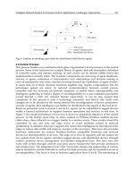
grammatically in Figure 11.6.
In Figure 11.6 the marginal cost curve is labeled MC. According to Equa-

tion (11.47) the firm should produce Q
1
units where marginal cost is equal
to the sum of MR
1
and MR
2
. The amount of Q
2
produced is proportional
to Q
1
.At that output level the firm charges P
1
for Q
1
and P
2
for Q
2
. It should
be noted that beyond output level Q
1
* in Figure 11.6, MR
2
becomes nega-
tive and MR
1+2
becomes simply MR
1

.
Suppose that marginal cost increases to MC¢. In this case, the firm should
produce Q
1
¢, but still only sell Q
1
* units. Any output in excess of Q
1
* should
be disposed of, since the firm’s marginal revenue beyond Q
1
* is negative.
The amount of Q
2
produced will be in fixed proportion to Q
1
¢. The price of
Q
1
* is P
2
¢ and the price of Q
2
is P
1
¢.
Problem 11.15. Suppose that a firm produces two units of Q
2
for each unit
of Q

1
. Suppose further that the demand equations for these two goods are
MR Q MR Q MC Q
11 21 1
()
+
()
=
()
dTR
dQ
dTR
dQ
dTC
dQ
1
1
2
1
1
1
+=
d
dQ
dTR
dQ
dTR
dQ
dTC
dQ

p
1
1
1
2
1
1
1
0=+-=
multiproduct pricing 457
FIGURE 11.6 Optimal pricing of two goods
jointly produced in fixed proportions with inde-
pendent demands.
The total cost of production is
a. What are the profit-maximizing output levels and prices for Q
1
and Q
2
?
b. At the profit-maximizing output levels, what is the firm’s total profit?
Solution
a. Solving the demand equations for P
1
and P
2
yields
The firm’s total profit equation is
Since Q
2
= 2Q

1
, this may be rewritten as
The first-order condition for profit maximization is
The second-order condition for profit maximization is
Since d
2
p/dQ
1
2
=-137 the second-order condition is satisfied. Solving the
first-order condition for Q
1
yields
The profit-maximizing level of Q
2
is
Substituting these results into the price equations yield
QQ
21
2328**.==
Q
1
164*.=
d
dQ
2
1
2
0
p

<
d
dQ
Q
p
1
1
220 134 0=- =
p= - +
()
-
()
+
()
=- - -
20 2 100 2 5 2 10 5 2
10 220 67
11
2
11
2
11
2
11
2
QQ Q Q QQ
QQ
p= + - +
()
=-

()
+-
()
-+
()
=-+ +
()
PQ PQ TC Q Q
QQ QQ Q
QQ QQ QQ
11 22 1 2
11 2 2
2
11
2
22
2
12
2
20 2 100 5 10 5
20 2 100 5 10 5
PQ
22
100 5=-
PQ
11
20 2=-
TC Q=+10 5
2
QP

22
20 0 2=
QP
11
10 0 5=
458 pricing practices
b. The firm’s total profit is
Problem 11.16. Suppose that a firm jointly produces two goods. Good B
is a by-product of the production of good A. The demand equations for the
two goods are
The firm’s total cost equation is
a. What is the profit-maximizing price for each product?
b. What is the firm’s total profit?
Solution
a. Solving the demand equation for price yields
The respective total and marginal revenue equations are
The firm’s marginal revenue equation is
The firm’s marginal cost equation is
The profit-maximizing rate of output is
MR MC=
MC
dTC
dQ
Q==+15 0 1.
MR MR MR Q Q Q
AB A B
=+=- +- =-20 0 2 24 0 4 44 0 6
MR Q
BB
=-24 0 4.

TR Q Q
BBB
=-24 0 2
2
.
MR Q
A
A
=-20 0 2.
TR Q Q
AAA
=-20 0 1
2
.
PQ
BB
=-24 0 2.
PQ
AA
=-20 0 1.
TC Q Q=+ +500 15 0 05
2
.
QP
BB
=-120 5
QP
AA
=-200 10
p=

()
-
()
-= - -=220 1 64 67 1 64 10 360 80 180 20 10 170 60
2
$.
P
2
100 5 3 28 83 60*.$.=-
()
=
P
1
20 2 1 64 16 72*.$.=-
()
=
multiproduct pricing 459
The profit-maximizing prices for the two goods are
b. The firm’s total profit is
PEAK-LOAD PRICING
In many markets the demand for a service is higher at certain times than
at others. The demand for electric power, for example, is higher during the
day than at night, and during summer and winter than during spring and
fall. The demand for theater tickets is greater at night and on the weekends
or for midweek matinees.Toll bridges have greater traffic during rush hours
than at other times of the day. The demand for airline travel is greater
during holiday seasons than at other times. During such “peak” periods it
becomes difficult, if not impossible, to satisfy the demands of all customers.
Thus the profit-maximizing firm will charge a higher price for the product
during “peak” periods and a lower price during “off-peak” periods. This

kind of pricing scheme is known as peak-load pricing.
Definition: Peak-load pricing is the practice of charging a higher price
for a service when demand is high and capacity is fully utilized and a lower
price when demand is low and capacity is underutilized.
Figure 11.7 illustrates an example of peak-load pricing for a profit-
maximizing firm. Here the marginal cost of providing a service is assumed
to be constant until capacity is reached at a peak output level of O
p
. At the
peak output level the marginal cost curve becomes vertical. This reflects
the fact that to satisfy additional demand at O
p
, the firm must increase its
capacity, by building a new bridge, installing a new hydroelectric generator,
or other high-cost measure.
The short-run production function is typically defined in terms of a time
interval over which certain factors of production are “fixed.” Strictly speak-
ing, this assertion is incorrect.In principle, virtually any factor may be varied
if the derived benefits are great enough. It is certainly the case, however,
that some factors of production are more easily varied that others. It is
clearly easier and less expensive to hire an additional worker at a moment’s
p* **** *.*
.
$, .
=+-++
()
=
()
+
()

()
+
()
[]
=
PQ PQ Q Q
AB
500 15 0 05
15 86 41 43 15 71 41 43 500 15 41 43 0 05 41 43
1 343 57
2
2
P
B
* .$.=-
()
=- =20 0 2 41 43 24 8 29 15 71
P
A
* .$.=-
()
=- =20 0 1 41 43 20 4 14 15 86
Q*.= 41 43
44 0 6 15 0 1-=+ QQ
460 pricing practices
notice than to build a new bridge. Thus, it is reasonable to assume that the
short-run marginal cost of expanding bridge traffic or increasing hydro-
electric capacity is infinite. For that reason, the marginal cost curve at Q
p

is
assumed to be vertical.
To maximize profits subject to capacity limitations, the firm will charge
different prices at different times. Off-peak prices are determined by equat-
ing marginal revenue to marginal operating costs. Peak prices, on the other
hand, are determined by equating marginal revenue to the marginal cost of
increasing capacity.In Figure 11.7, for example, MR = MC for off-peak users
at output level Q
op
. At that output level the firm will charge off-peak users
a price of P
op
. On the other hand, the profit-maximizing level of output for
peak users is at the firm’s capacity, which in Figure 11.7 occurs at output
level Q
p
. At that output level the marginal cost curve of producing the
service becomes vertical. The profit-maximizing price at that output level is
P
p
.
Peak-load pricing suggests that users of, say, congested bridges during
rush hours, ought to be charged a higher toll than users during non–rush
hour periods when there is excess capacity. Since peak-period demand
strains capacity, the cost of additional capital investment ought to be borne
by peak-period users. This tends to run contrary to the common practice
on trains and toll bridges of offering multiple-use discounts to commuters
traveling during rush hour, such as lower per-ride prices for, say, monthly
tickets on commuter railways.
Problem 11.17. The Gotham Bridge and Tunnel Authority (GBTA) has

estimated the following demand equations for peak and off-peak auto-
mobile users of the Frog’s Neck Bridge:
Peak:
Off-peack:
TQ
op op
=-5005.
TQ
pp
=-10 0 02.
peak-load pricing 461
FIGURE 11.7 Peak-load pricing.