Managerial economics theory and practice phần 8 doc

Consider again the cash flows for projects A and B summarized in Table
12.1. Also assume that the cost of capital (k) is 10%. To determine the net
present value of each project, simply divide the cash flow for each period
by (1 + k)
t
. The calculation for the net present value of project A (NPV
A
)
is illustrated in Figure 12.13 as $1,109.13. It can just as easily be illustrated
that the net present value of project B is $94.95.
Table 12.4 compares the net present values of projects A and B. If the
two are independent, then both investments should be undertaken. On the
other hand, if projects A and B are mutually exclusive, then project A will
be preferred to project B because its net present value is greater.
A positive net present value indicates that the project is generating cash
flows in excess of what is required to cover the cost of capital and to provide
a positive rate of return to investors. Finally, if the net present value is neg-
ative, the present value of cash inflows is not sufficient to cover the present
value of cash outflows.A project should not be undertaken if its net present
value is negative.
512 Capital Budgeting
+
0
12345t
k = 0.10
Ϫ$25,000.00
9,090.91
6,611.57
4,507.89
2,483.69
Ϫ$1,109.13 = NPV

A
$10,000 $8,000 $6,000 $5,000 $4,000
3,415.07
Ϫ
FIGURE 12.13 Net present value calculations for project A.
TABLE 12.4 Net Present Value (NPV)
for Projects A and B
Year, t Project A Project B
0 -$25,000.00 -$25,000.00
1 9,090.91 2,727.27
2 6,611.57 4,132.23
3 4,507.89 5,259.20
4 3,415.07 6,146.12
5 2,483.69 6,830.13
S $1,109.13 $94.95
Problem 12.12. Illuvatar International pays the top corporate income tax
rate of 38%. The company is planning to build a new processing plant to
manufacture silmarils on the outskirts of Valmar, the ancient capital of
Valinor. The new plant will require an immediate cash outlay of $3 million
but is expected to generate annual profits of $1 million. According to the
Valinor Uniform Tax Code, Illuvatar may deduct $500,000 in taxes annu-
ally as depreciation. The life of the new plant is 5 years. Assuming that the
annual interest rate is 10%, should Illuvatar build the new processing plant?
Explain.
Solution. According to the information provided, Illuvatar’s taxable return
is R
t
=p
t
- D

t
, where p
t
represents profits and D
t
is the amount of depreci-
ation that may be deducted in period t for tax purposes. Illuvatar’s taxable
rate of return is
Illuvatar’s annual tax (T
t
) is given as T
t
=tR
t
, where t is the tax rate.
Illuvatar’s annual tax is, therefore,
Illuvatar’s after tax income flow (p
t
*) is given as
At an interest rate of 10%, the net present value of the after tax income
flow is given as
where O
0
= $3,000,000, the initial cash outlay. Substituting into this expres-
sion, we obtain
Because the net present value is positive, Illuvatar should build the new
processing plant.
Problem 12.13. Senior management of Bayside Biotechtronics is con-
sidering two mutually exclusive investment projects. The projected net
cash flows for projects A and B are summarized in Table 12.5. If the dis-

count rate (cost of capital) is expected to be 12%, which project should be
undertaken?
NPV =
()
+
()
+
()
+
()
+
()
-
=
810 000
110
810 000
110
810 000
110
810 000
110
810 000
110
3 000 000
70 537 29
2345
,
.
,

.
,
.
,
.
,
.
,,
$, .
NPV
i
O
i
ttt t
=
+
()
-
+
()
=Æ =Æ
SS
15
5
00
0
11
p *
pp
ttt

T* $,, $, $,=-= - =1 000 000 190 000 810 000
T
t
=
()
=0 38 500 000 190 000.,$,
R
t
=-=$, , $ , $ ,1 000 000 500 000 500 000
Methods for Evaluating Capital Investment Projects 513
Solution
a. The net present value of project A and project B are calculated as
Since NPV
B
> NPV
A
, project B should be adopted by Bayside.
Sometimes, mutually exclusive investment projects involve only cash out-
flows. When this occurs, the investment project with the lowest absolute net
present value should be selected, as Problem 12.14 illustrates.
Problem 12.14. Finn MacCool, CEO of Quicken Trees Enterprises, is con-
sidering two equal-lived psalter dispensers for installation in the employee’s
recreation room. The projected cash outflows for the two dispensers are
summarized in Table 12.6. If the cost of capital is 10% per year and
dispense A and B have salvage values after 5 years of $200 and $350,
respectively, which dispenser should be installed?
Solution. The net present values of dispenser A and dispenser B are
calculated as
NPV
CF

k
CF
k
CF
k
CF
k
A
=
+
()
+
+
()
+
+
()
++
+
()
=
-
()
-
()
-
()
-
()
-

()
-
()
+
()
=-
0
0
1
1
2
2
5
5
0123455
111 1
2 500
110
900
110
900
110
900
110
900
110
900
110
200
110

5 787 53

,

$, .
NPV
B
=
-
()
+
()
+
()
+
()
+
()
+
()
=
19 000
112
6 000
112
6 000
112
6 000
112
6 000

112
6 000
112
2 628 66
0 12345
,
.
,
.
,
.
,
.
,
.
,
.
$, .
NPV
CF
k
CF
k
CF
k
CF
k
A
n
=

+
()
+
+
()
+
+
()
++
+
()
=
-
()
+
()
+
()
+
()
+
()
+
()
=
0
0
1
1
2

25
0 12345
111 1
25 000
112
7 000
112
8 000
112
9 000
112
9 000
112
5 000
112
2 590 36

,
.
,
.
,
.
,
.
,
.
,
.
$, .

514 Capital Budgeting
TABLE 12.5 Net Cash Flows (CF
t
) for
Projects A and B
Year, t Project A Project B
0 -$25,000 -$19,000
1 7,000 6,000
2 8,000 6,000
3 9,000 6,000
4 9,000 6,000
5 5,000 6,000
Since |NPV
A
| < |NPV
B
|, Finn MacCool will install dispenser A.
Problem 12.15. Suppose that an investment opportunity, which requires
an initial outlay of $50,000, is expected to yield a return of $150,000 after
20 years.
a. Will the investment be profitable if the cost of capital is 6%?
b. Will the investment be profitable if the cost of capital is 5.5%?
c. At what cost of capital will the investor be indifferent to the investment?
Solution
a. The net present value of the investment with a cost of capital of 6% is
given as
Since the net present value is negative, we conclude that the investment
opportunity is not profitable.
b. The net present value of the investment with a cost of capital of 5.5% is
Since the net present value is positive, we can conclude that the invest-

ment opportunity is profitable.
c. The investor will be indifferent to the investment if the net present value
is zero. Substituting NPV = 0 into the expression and solving for the
discount rate yields
NPV =
()
-= -=
150 000
1 055
50 000
150 000
292
50 000 1 409 34
20
,
.
,
,
.
,$,.
NPV =
()
-= -=-
150 000
106
50 000
150 000
321
50 000 3 229 29
20

,
.
,
,
.
,$,.
NPV
B
=
-
()
-
()
-
()
-
()
-
()
-
()
+
()
=-
3 500
110
700
110
700
110

700
110
700
110
700
110
350
110
5 936 23
0123455
,

$, .
Methods for Evaluating Capital Investment Projects 515
TABLE 12.6 Net Cash Flows (CF
t
) for
Dispensers A and B
Year, t Dispenser A Dispenser B
0 -$2,500 -$3,500
1 -900 -700
2 -900 -700
3 -900 -700
4 -900 -700
5 -900 -700
That is, the investor will be indifferent to the investment at a cost of
capital of approximately 5.65%.
NET PRESENT VALUE (NPV) METHOD FOR
UNEQUAL-LIVED PROJECTS
Whereas comparing alternative investment projects with equal lives is a

fairly straightforward affair, how do we compare projects that have differ-
ent lives? Since net present value comparisons involve future cash flows, an
appropriate analysis of alternative capital projects must be compared over
the same number of years. Unless capital projects are compared over an
equivalent number of years, there will be a bias against shorter lived capital
projects involving net cash outflows, and a bias in favor of longer lived
capital projects involving net cash inflows. To avoid this time and cash flow
bias when one is evaluating projects with different lives, it is necessary to
modify the net present value calculations to make the projects comparable.
A fair comparison of alternative capital projects requires that net present
values be calculated over equivalent time periods. One way to do this is to
compare alternative capital projects over the least common multiple of
their lives. To accomplish this, the cash flows of each project must be dupli-
cated up to the least common multiple of lives for each project. By artifi-
cially “stretching out” the lives of some or all of the prospective projects
until all projects have the same life span, we can reduce the evaluation of
capital investment projects with unequal lives to a straightforward applica-
tion of the net present value approach to evaluating projects discussed in
the preceding section. In problem 12.16, for example, project A has a life
expectancy of 2 years, while project B has a life expectancy of 3 years. To
compare these two projects by means of the net present value approach,
project A will be replicated three times and project B will be replicated
twice. In this way, both projects will have a 6-year life span.
Problem 12.16. Brian Borumha of Cashel Company, a leading Celtic oil
producer, is considering two mutually exclusive projects, each involving
drilling operations in the North Sea. The projected net cash flows for each
project are summarized in Table 12.7. Determine which project should be
adopted if the cost of capital is 8%.
0
150 000

1
50 000
50 000 1 150 000
13
1 1 05646
0 05647
20
20
20
=
+
()
-
+
()
=
+
()
=
+=
=
,
,
,,
.
.
k
k
k
k

k
516 Capital Budgeting
Solution. Since the projects have different lives, they must be compared
over the least common multiple of years, which in this case is 6 years.
Since NPV
B
> NPV
A
, Brian Borumha will select project B over project A.
INTERNAL RATE OF RETURN (IRR) METHOD
AND THE HURDLE RATE
Yet another method of evaluating a capital investment project is by cal-
culating the internal rate of return (IRR). Before discussing the methodol-
ogy of calculating a project’s internal rate of return, it is important to
understand the rationale underlying this approach. Consider, for example,
the case of an investor who is considering purchasing a 12-year, 10% annual
coupon, $1,000 par-value corporate bond for $1,150.70. Before deciding
whether the investor should purchase this bond, consider the following
definitions.
Coupon bonds are debt obligations of private companies or public agen-
cies in which the issuer of the bond promises to pay the bearer of the bond
a series of fixed dollar interest payments at regular intervals for a specified
NPV
B
=
-
()
+
()
+

()
+
()
-
()
+
()
+
()
+
()
=
5 000
108
1 000
108
2 500
108
3 000
108
5 000
108
1 000
108
2 500
108
3 000
108
808 61
01233

456
,
.
,
.
,
.
,
.
,
.
,
.
,
.
,
.
$.
NPV
CF
k
CF
k
CF
k
CF
k
A
=
+

()
+
+
()
+
+
()
++
+
()
=
-
()
+
()
+
()
-
()
+
()
+
()
-
()
0
0
1
1
2

2
6
6
012234
111 1
2 000
108
1 000
108
1 500
108
2 000
108
1 000
108
1 500
108
2 000
108

$,
.
$,
.
$,
.
$,
.
,
.

,
.
,
.
4456
1 000
108
1 500
108
549 41
+
()
+
()
=
,
.
,
.
$.
Methods for Evaluating Capital Investment Projects 517
TABLE 12.7 Net Cash Flows (CF
t
) for
Projects A and B ($ millions)
Year, t Project A Project B
0 -$2,000 -$5,000
1 1,000 1,000
2 1,500 2,500
3 3,000

period of time. Upon maturity, the issuer agrees to repay the bearer the par
value of the bond. The par value of a bond is the face value of the bond,
which is the amount originally borrowed by the issuer. Thus, a corporation
that issues a $1,000 coupon bond is obligated to pay the bearer of the bond
fixed dollar payments at regular intervals. In the present example, the issuer
of the bond promises to pay the bearer of the bond $100 per year for the
next 12 years plus the face value of the bond at maturity. Parenthetically,
the term “coupon bond” comes from the fact that at one time a number of
small, dated coupons indicating the amount of interest due to the owner
were attached to the bonds. A bond owner would literally clip a coupon
from the bond on each payment date and either cash or deposit the coupon
at a bank or mail it to the corporation’s paying agent, who would then send
the owner a check in the amount of the interest.
Definition: Coupon bonds are debt obligations in which the issuer of the
bond promises to pay the bearer of the bond fixed dollar interest payments
at regular intervals for a specified period of time, with reimbursement of
the face value at the end of the period.
Definition: The par value of a bond is the face value of the bond. It is
the amount originally borrowed by the issuer.
Why would an investor consider purchasing a bond for an amount in
excess of its par value? The reason is simple. In the present example, when
the bond was first issued the prevailing rate of interest paid on bonds with
equivalent risk and maturity characteristics was 10%. If the bond holder
wanted to sell the bond before maturity, the market price would reflect the
prevailing rate of interest.
If current market interest rates are higher than the coupon interest rate,
the bearer will have to sell the bond at a discount from par value. Other-
wise, no one would be willing to buy such a bond. On the other hand, if pre-
vailing interest rates are lower than the coupon interest rate, then the bearer
will be able to sell the bond at a premium. The size of the discount or

premium reflects the term to maturity and the differential between the pre-
vailing market interest rate and the coupon rate on bonds with similar risk
characteristics. Since the market value of the bond in the present example
is greater than its par value, prevailing market rates must be lower than the
coupon interest rate.
Returning to our example, should the investor purchase this bond? The
decision to buy or not to buy this bond will be based upon the rate of return
the investor will earn on the bond if held to maturity. This rate of return is
called the bond’s yield to maturity (YTM). If the bond’s YTM is greater than
the prevailing market rate of interest, the investor will purchase the bond.
If the YTM is less than the market rate, the investor will not purchase. If
the YTM is the same as the market rate, other things being equal, the
investor will be indifferent between purchasing this bond and a newly
issued bond.
518 Capital Budgeting
Definition: Yield to maturity is the rate of return earned on a bond that
is held to maturity.
Calculating the bond’s YTM involves finding the rate of interest that
equates the bond’s offer price, in this case $1,150.70,to the net present value
of the bond’s cash inflows. Denoting the value price of the bond as V
B
,the
interest payment as PMT, and the face value of the bond as M, the yield to
maturity can be found by solving Equation (12.27) for YTM.
(12.27)
Substituting the information provided into Equation (12.27) yields
Unfortunately, finding the YTM that satisfies this expression is easier
said than done. Different values of YTM could be tried until a solution
is found, but this brute force approach is tedious and time-consuming.
Fortunately, financial calculators are available that make the process of

finding solution values to such problems a trivial procedure. As it turns out,
the yield to maturity in this example is YTM* = 0.08, or an 8% yield to
maturity. The solution to this problem is illustrated in Figure 12.14.
$, .
$$

$$,
1 150 72
100
1
100
1
100
1
1 000
1
12
=
+
()
+
+
()
++
+
()
+
+
()
YTM YTM YTM YTM

nn
V
PMT
YTM
PMT
YTM
PMT
YTM
M
YTM
PMT
YTM
M
YTM
B
nn
tn
tn
=
+
()
+
+
()
++
+
()
+
+
()

=
+
()
+
+
()
=Æ
11 1 1
11
12
1

S
Methods for Evaluating Capital Investment Projects 519
+
Ϫ
12345 t
YTM = 0.08
6789
10 11 12
$100 $100 $100 $100 $100 $100 $100 $100 $100 $100 $100
$1,000
$100
$92.539
85.733
79.383
73.503
68.058
63.017
58.349

54.027
50.025
46.319
42.888
39.711
397.114
$1,150.720 =V
B
FIGURE 12.14 Yield to maturity.
Thus, the investor will compare the YTM to the rate of return on bonds of
equivalent risk characteristics before deciding whether to purchase the
bond. Parenthetically, the efficient markets hypothesis suggests that the
YTM on this coupon bond will be the same as the prevailing market
interest rate.
We now return to the internal rate of return method for evaluating
capital projects, introduced earlier. As we will see shortly, the methodology
for determining the yield to maturity on a bond is the same as that used for
calculating the internal rate of return. The internal rate of return is the dis-
count rate that equates the present value of a project’s expected cash
inflows with the project’s expected cash outflows.The internal rate of return
may be calculated from Equation (12.28).
(12.28)
Consider, again, the information presented in Table 12.1 for project A.
This problem is illustrated in Figure 12.15.
To determine the discount rate for which NPV is zero, substitute the
information provided for project A in Table 12.1 into Equation (12.27),
which yields
NPV
IRR IRR IRR
IRR IRR

=- +
+
()
+
+
()
+
+
()
+
+
()
+
+
()
=
$,
$ , $, $,
$, $,
25 000
10 000
1
8 000
1
6 000
1
5 000
1
4 000
1

0
123
45
NPV CF
CF
IRR
CF
IRR
CF
IRR
CF
IRR
n
n
tnt
t
=+
+
()
+
+
()
++
+
()
=
+
()
=
=Æ

0
1
1
2
2
1
11 1
1
0

S
520 Capital Budgeting
+
0
12 3 4 5t
IRR =?
Ϫ$25,000.00
NPV=0
$10,000 $8,000 $6,000
$5,000 $4,000
͕
⌺
t=1Ł5
PV
i
=
$25,000.00
_________
–
FIGURE 12.15 Internal rate of return is the discount rate for which the net present value

of a project is equal to zero.
Of course, finding IRR is no easier than solving for YTM, as discussed
earlier. Once again, a financial calculator comes to the rescue. The internal
rate of return for projects A and B are IRR
A
= 12.05% and IRR
B
= 10.12%.
Whether these projects are accepted or rejected depends on the cost of
capital, which is sometimes referred to as the hurdle rate, required rate of
return, or cutoff rate. The somewhat colorful expression “hurdle rate” is
meant to express the notion that a company can increase its shareholder
value by investing in projects that earn a rate of return that exceeds (hurdles
over) the cost of capital used to finance the project.
Definition: The internal rate of return is the discount rate that equates
the present value of a project’s expected cash inflows with the project’s
expected cash outflows.
Definition: The hurdle rate is the cost of capital of a project that must
be exceeded by the internal rate of return if the project is to be accepted.
Often referred to as the required rate of return or the cutoff rate.
Another way to look at the internal rate of return is that it is the
maximum rate of interest that an investor will pay to finance a capital
investment project.Alternatively, the internal rate of return is the minimum
acceptable rate of return on an investment. Thus, if the internal rate of
return is greater than the cost of capital (hurdle rate), a project will be
accepted. If the internal rate of return is less than the hurdle rate, a project
will be rejected. Finally, if the internal rate of return is equal to the cost of
capital, the investor will be indifferent to the project. Of course, the investor
would like to earn as much as possible in excess of the internal rate of
return.

Suppose that an investor is considering investing in either project A or
project B. If the two projects are independent and the internal rate of return
exceeds the hurdle rate, both projects will be accepted. On the other hand,
if the projects are mutually exclusive, project A will be preferred to project
B because of its higher internal rate of return.The NPV and IRR will always
result in the same accept and reject decisions for independent projects. This
is because, by definition, when NPV is positive, then IRR will exceed the
cost of funds to finance the project. On the other hand, the NPV and IRR
methods can result in conflicting accept/reject decisions for mutually exclu-
sive projects. A comparison of the NPV and IRR methods of evaluating
capital investment projects will be the subject of the next section.
Problem 12.17. Consider, again, Bayside Biotechtronics. The projected net
cash flows for projects A and B are summarized in Table 12.8.
a. Calculate the internal rate of return for both projects.
b. If the cost of capital for financing the projects (hurdle rate) is 17%, which
project should be considered?
c. Verify that if the hurdle rate is 1% lower, NPV
A
> 0
d. Verify that if the hurdle rate is 1% higher, NPV
B
< 0.
Methods for Evaluating Capital Investment Projects 521
Solution
a. To determine the internal rate of return for projects A and B, substitute
the information provided in the table into the Equation (12.27) and solve
for IRR.
Since calculating IRR
A
and IRR

B
by trial and error is time-consuming
and tedious, the solution values were obtained by using a financial cal-
culator. The internal rates of return for projects A and B are
b. The internal rate of return is less than the hurdle rate for project A and
greater than the hurdle rate for project B. Thus, project A is rejected and
project B is accepted.
c. Substituting into Equation (12.28), we write
IRR
IRR
A
B
=
=
16 168
17 448
.%
.%
NPV
IRR IRR IRR
IRR IRR
B
BB B
BB
=- +
+
()
+
+
()

+
+
()
+
+
()
+
+
()
=
$,
$, $, $,
$, $,
19 000
6 000
1
6 000
1
6 000
1
6 000
1
6 000
1
0
123
45
NPV CF
CF
IRR

CF
IRR
CF
IRR
IRR IRR IRR
IRR IRR
A
AA A
AA A
AA
=+
+
()
+
+
()
++
+
()
=- +
+
()
+
+
()
+
+
()
+
+

()
+
+
()
=
0
1
1
2
2
5
5
123
45
11 1
25 000
7 000
1
8 000
1
9 000
1
9 000
1
5 000
1
0

$,
$, $, $,

$, $,
522 Capital Budgeting
TABLE 12.8 Net Cash Flows CF
t
for
Projects A and B
Year, t Project A Project B
0 -$25,000 -$19,000
1 7,000 6,000
2 8,000 6,000
3 9,000 6,000
4 9,000 6,000
5 5,000 6,000
d.
COMPARING THE NPV AND IRR METHODS
Consider, once again, the cash flows for projects A and B presented in
Table 12.1. Table 12.9 summarizes the net present values for the cash flows
of project A and B for different costs of capital. The data summarized in
Table 12.9 are illustrated in Figure 12.16. A diagram that plots the rela-
tionship between the net present value of a project and alternative costs of
capital is called a net present value profile.
Definition: A net present value profile is a diagram that shows the rela-
tionship between the net present value of a project and alternative costs of
capital.
When the cost of capital is zero, the project’s net present value is simply
the sum the project’s net cash flows. In the present example, the net present
values for projects A and B when k = 0.00% are $8,000 and $10,000, respec-
tively. The student will also readily observe from Equation (12.28) that as
the cost of capital increases, the net present value of the project declines,
which gives rise to the downward-sloping curves in Figure 12.16.

NPV
CF
A
tnt
t
=
()
=-
=Æ
S
1
1 17168
563 64
.
$.
NPV
CF
A
tnt
t
=
()
=- +
()
+
()
+
()
+
()

+
()
=
=Æ
S
1
123
45
1 15168
25 000
7 000
1 15168
8 000
1 15168
9 000
1 15168
9 000
1 15168
5 000
1 15168
584 85
.
$,
$,
.
$,
.
$,
.
$,

.
$,
.
$.
Methods for Evaluating Capital Investment Projects 523
TABLE 12.9 Net Present Value Profiles
for Projects A and B
Cost of capital Project A Project B
0.00 $8,000 $10,000
0.02 6,389 7,621
0.04 4,908 5,465
0.05 4,211 4,462
0.05875 3,623 3,623
0.06 3,541 3,506
0.08 2,278 1,723
0.10 1,109 96
0.12 24 -1,392
0.14 -985 -2,755
In one earlier discussion, the internal rate of return was defined as the
discount rate at which the NPV of a project is zero. For projects A and B,
the internal rates of return (not shown in Table 12.9) are 12.05 and 10.12%,
respectively. These values are illustrated in Figure 12.16 at the points at
which the net present value profiles for projects A and B intersect the
horizontal axis.
The student will note that when the cost of capital is 5.875%, the net
present values of projects A and B are the same. Additionally, when the cost
of capital is less than 5.875% NPV
A
< NPV
B

, and when the cost of capital
is greater than 5.875% NPV
A
> NPV
B
. This is illustrated in Figure 12.14 at
the point of intersection of the present value profiles of project A and B.
For obvious reasons, the cost of capital at which the NPVs of two projects
are equal is called the crossover rate.
Definition: The crossover rate is the cost of capital at which the net
present values of two projects are equal. Diagrammatically, this is the cost
of capital at which the net present value profiles of two projects intersect.
An examination of Figure 12.16 also reveals that the marginal change in
NPV
B
given a change in the cost of capital is greater than that for NPV
A
(i.e., ∂NPV
B
/∂k >∂NPV
A
/∂k). In other words, the slope of the net present
value profile for project B is steeper than the net present value profile for
project A. The reason for this is that project B is more sensitive to changes
in the cost of capital than project A.
Given the cost of capital, the sensitivity of NPV to changes in the cost
of capital will depend on the timing of the project’s cash flows. To see this,
consider once again the cash flows summarized in Table 12.1. Note that
these cash flows are received more quickly in the case of project A than for
project B. Referring to Table 12.9, when the cost of capital is doubled from

5.0% to 10.0%, NPV
A
falls from $4,211 to $1,109, or a decline of 73.7%. For
project B, NPV
B
falls from $4,462 to $96, or a drop of 97.8%. The reason
for the discrepancy is the discounting factor 1/(1 + k)
n
, which will be greater
524 Capital Budgeting
NPV
$10,000
$8,000
$3,623
0
NPV
B
profile
NPV
A
profile
Crossover
IRR
A
=12.05%
IRR
B
=10.12%
4.0 5.5875 8.0
k

14.0
FIGURE 12.16 Internal rates of return and crossover rate.
for cash flows received in the distant future than for cash flows received in
the near future. Thus, the net present value of projects that receive greater
cash flows in the distant future will decline at a faster rate than for projects
receiving most of their cash in the early years.
NPV AND IRR METHODS FOR INDEPENDENT
PROJECTS
It was noted earlier that when the cost of capital is less than IRR for both
projects, then the NPV and IRR methods will always result in the same
accept and reject decisions. This can be seen in Figure 12.16. If the cost of
capital is less than 10.12%, and projects A and B are independent, both pro-
jects will be accepted. If the cost of capital is between 10.12 and 12.05%,
project A will be accepted and project B will be rejected. Finally, If the cost
of capital is greater than 12.05%, then both projects will be rejected.
NPV AND IRR METHODS FOR MUTUALLY
EXCLUSIVE PROJECTS
We noted earlier that if the projects are mutually exclusive (the accep-
tance of one project means the rejection of the other), the NPV and IRR
methods can result in conflicting accept/reject decisions. To see this, con-
sider again Figure 12.16. If the cost of capital is greater than the crossover
rate, but less than IRR for both projects, in this case 10.12%, then NPV
A
>
NPV
B
and IRR
A
> IRR
B

, in which case both the IRR and NPV methods
indicate that project A is preferred to project B.
On the other hand, if the cost of capital is less than the crossover rate,
then although IRR
A
is still less than IRR
B
, NPV
B
> NPV
A
. Thus, the net
present value method indicates that project B should be preferred to
project A and the internal rate of return method ranks project B higher
than project A. In other words, when the cost of capital is less than the
crossover rate, a conflict arises between the NPV and IRR methods. Two
questions immediately present themselves:
1. Why do the net present value profiles intersect?
2. When an accept/reject conflict exists because the cost of capital is
less than the crossover rate, which method should be used to rank
mutually exclusive projects?
The net present value profiles of two projects may intersect for two
reasons: differences in project sizes and cash flow timing differences. As
noted earlier, the effect of discounting will be greater for cash flows
received in the distant future than for cash flows received in the near future.
The net present value of projects in which most of the cash flows are
received in the distant future will decline at a faster rate than the decline
in the net present value for projects in which most of the cash flows are
Methods for Evaluating Capital Investment Projects 525
generated in the near future. Thus, if the NPV for one project (project B in

Figure 12.16) is greater than the NPV for another project (project A in
Figure 12.16) when t = 0 and most of the cash flows for the first project are
received in the distant future in comparison to the second project, the net
present value profiles of the two projects may intersect.
When the net present value profiles intersect and the cost of capital is
less than the crossover rate, which method should be used for selecting a
capital investment project? The answer depends on the rate at which the
firm reinvests the net cash inflows over the life of the project. The NPV
method implicitly assumes that net cash inflows are reinvested at the cost
of capital. The IRR method assumes that net cash inflows are reinvested at
the internal rate of return. So, which of these assumptions is more realis-
tic? It may be demonstrated (see Brigham, Gapenski, and Erhardt 1998,
Chapter 11) that the best assumption is that a project’s net cash inflows are
reinvested at the firm’s cost of capital. Thus, for ranking mutually exclusive
capital investment projects, the NPV method is preferred to the IRR
method.
Problem 12.18. Consider, again, the net cash flows for projects A and B in
Bayside Biotechtronics, summarized in Table 12.10.
a. Illustrate the net present value profiles for projects A and B.
b. What is the crossover rate for the two projects?
c. Assuming that projects A and B are mutually exclusive, which project
should be selected if the cost of capital is greater than the crossover rate?
Which project should be selected if the cost of capital is less than the
crossover rate?
Solution
a. A financial calculator was used to find the net present values for pro-
jects A and B for various interest rates are summarized in Table 12.11.
To determine the crossover rate, using Equation (12.25) to equate the
net present value of project A with the net present value of project B
and solve for the cost of capital, k.

526 Capital Budgeting
TABLE 12.10 Net Cash Flows (CF
t
) for
Projects A and B
Year, t Project A Project B
0 -$25,000 -$19,000
1 7,000 6,000
2 8,000 6,000
3 9,000 6,000
4 9,000 6,000
5 5,000 6,000
Bringing all the terms in this expression to the left-hand side of the
equation, we get
The value for k in this expression may be found using the IRR function
of a financial calculator. Solving for k yields a crossover rate of 11.72%.
Last, the internal rates of return for projects A and B may be calcu-
lated from Equation (12.28).
Solving with a financial calculator yields
IRR
A
= 16 17.%
NPV CF
CF
IRR
CF
IRR
CF
IRR
IRR IRR IRR IRR

IRR IRR
A
n
=+
+
()
+
+
()
++
+
()
=
-
+
()
+
+
()
+
+
()
+
+
()
+
+
()
+
+

()
=
0
1
1
2
25
0123
45
11 1
25 000
1
7 000
1
8 000
1
9 000
1
9 000
1
9 000
1
0

$ , $, $, $,
$, $,
-
+
()
+

+
()
+
+
()
+
+
()
+
+
()
-
+
()
=
$, $, $, $, $, $,6 000
1
1 000
1
2 000
1
3 000
1
3 000
1
3 000
1
0
0 12345
kkkkkk

NPV NPV
kkkkkk
kkkk
AB
=
-
+
()
+
+
()
+
+
()
+
+
()
+
+
()
+
+
()
=
-
+
()
+
+
()

+
+
()
+
+
()
$ , $, $, $, $, $,
$ , $, $, $,
25 000
1
7 000
1
8 000
1
9 000
1
9 000
1
9 000
1
19 000
1
6 000
1
6 000
1
6 000
1
0 12345
0 123

++
+
()
+
+
()
$, $,6 000
1
6 000
1
45
kk
Methods for Evaluating Capital Investment Projects 527
TABLE 12.11 Net Present Value
Profiles for Projects A and B
Cost of capital Project A Project B
0.00 $13,000 $11,000
0.04 8,931 7,711
0.06 7,145 6,274
0.08 5,503 4,956
0.10 3,989 3,745
0.1172 2,780 2,780
0.12 2,590 2,629
0.14 1,296 1,598
0.16 97 646
0.18 -1,017 -237
Similarly for project B,
Solving,
Finally, using the crossover rate to calculate the net present value of
projects A and B yields

With this information, the net present value profiles for projects A and
B may be illustrated in Figure 12.17.
b. From Figure 12.17, the crossover rate for the two projects is 11.72%.
c. From Figure 12.17, if the cost of capital is greater than 11.72%, but less
than 16.17%, project B is preferred to project A because NPV
B
> NPV
A
.
This choice of projects is consistent with the IRR method, since IRR
B
>
NPV
B
=
-
()
+
()
+
()
+
()
+
()
+
()
=
$,
.

$,
.
$,
.
$,
.
$,
.
$,
.
$,
19 000
1 1172
6 000
1 1172
6 000
1 1172
6 000
1 1172
6 000
1 1172
6 000
1 1172
2 780
0123
45
NPV
A
=
-

()
+
()
+
()
+
()
+
()
+
()
=
$,
.
$,
.
$,
.
$,
.
$,
.
$,
.
$, .
25 000
1 1172
7 000
1 1172
8 000

1 1172
9 000
1 1172
9 000
1 1172
9 000
1 1172
5 077 91
0123
45
IRR
B
= 17 45.%
NPV
IRR IRR IRR IRR
IRR IRR
B
=
-
+
()
+
+
()
+
+
()
+
+
()

+
+
()
+
+
()
=
$ , $, $, $,
$, $,
19 000
1
6 000
1
6 000
1
6 000
1
6 000
1
6 000
1
0
0123
45
528 Capital Budgeting
NPV
$13,000
$11,000
$2,780
0

NPV
B
profile
NPV
A
profile
Crossover
IRR
A
= 16.17%
IRR
B
= 17.45%
k
11.72%
FIGURE 12.17 Diagrammatic solution to problem 12.18, parts b and c.
IRR
A
. On the other hand, if the cost of capital is less than 11.72%, project
A is preferred to project B, since NPV
A
> NPV
B
.This result conflicts with
the choice of projects indicated by the IRR method.
MULTIPLE INTERNAL RATES OF RETURN
In addition to the problems associated with using the IRR method for
evaluating capital investment projects, there is yet another potential fly in
the ointment: a project may have multiple internal rates of return.
Definition: A project with two or more internal rates of return is said to

have multiple internal rates of return.
To illustrate how multiple internal rates of return might occur, consider
again Equation (12.28) for calculating the net present value of a project.
(12.28)
The student will immediately recognize that Equation (12.28) is a poly-
nomial of degree n. What this means is that depending on the values of CF
t
,
Equation (12.28) may have n possible solutions for the internal rate of
return! Before discussing the conditions under which multiple internal rates
of return are possible, consider Table 12.12, which summarizes the cash
flows of a capital investment project.
Substituting the cash flow information from Table 12.12 into Equation
(12.28), we obtain
(12.29)
Equation (12.29) is a second-degree polynomial (quadratic) equation,
which may have two solution values. To find the solution values, rewrite
Equation (12.29) as
-
+
Ê
Ë
ˆ
¯
+
+
Ê
Ë
ˆ
¯

-=$, $, $,6 000
1
1
6 000
1
1
1 000 0
2
IRR IRR
NPV
IRR IRR
=- +
+
()
-
+
()
=$,
$, $,
1 000
6 000
1
6 000
1
0
12
NPV CF
CF
IRR
CF

IRR
CF
IRR
CF
IRR
n
n
tnt
t
=+
+
()
+
+
()
++
+
()
=
+
()
=
=Æ
0
1
1
2
2
1
11 1

1
0

S
Methods for Evaluating Capital Investment Projects 529
TABLE 12.12 Net Cash Flows (CF
t
) for
Project A
Year, tCF
t
0 -$1,000
1 6,000
2 -6,000
which is of the general form
(2.69)
The solution values may be found by applying the quadratic equation
(2.70)
Substituting the information provided in Equation (12.29) into Equation
(2.70) yields
The solution values are
We find that for the cash flows summarized in Table 12.12, this project
has internal rates of return of both 27 and 476%. The NPV profile for this
project is summarized in Table 12.13 and Figure 12.18.
Under what circumstances are multiple internal rates of return possible?
Thus, far we have dealt only with normal cash flows. A project has normal
cash flows when one or more of the cash outflows are followed by a series
of cash inflows. The cash flow depicted in Table 12.12 is an example of an
abnormal cash flow. A large cash outflow during or toward the end of the
life of a project is considered to be abnormal. Projects with abnormal cash

flows may exhibit multiple internal rates of return.
Definition: A project has a normal cash flow if one or more cash out-
flows are followed by a series of cash inflows.
1
1
6 000 3 464 10
12 000
021
1476
376
1
1
6 000 3 464 10
12 000
079
1127
027
1
1
1
2
2
2
+
Ê
Ë
ˆ
¯
=

-
=
+
()
=
=
+
Ê
Ë
ˆ
¯
=
-+
-
=
+
()
=
=
IRR
IRR
IRR
IRR
IRR
IRR
,,.
,
.
.
.

,,.
,
.
.
.
1
1
6 000 6 000 4 6 000 1 000
2 6 000
6 000 36 000 000 24 000 000
12 000
6 000 12 000 000
12 000
6 000 3 464 10
12 000
12
2
05
05
05
+
Ê
Ë
ˆ
¯
=
-±
()

()

-
()
[]
-
()
=
-± -
[]
-
=
-±
()
-
=
-±
-
IRR
,
.
.
.
,, ,,
,
,,,,,
,
,,,
,
,,.
,
x

bb ac
a
12
2
05
4
2
,
.
=
-± -
()
ax bx c
2
0++=
530 Capital Budgeting
Definition: A project has an abnormal cash flow when large cash out-
flows occur during or toward the end of the project’s life.
As before, no difficulties arise when the net present value method is used
to evaluate capital investment projects. In our example, if the cost of capital
is between 27 and 376% independent projects should be accepted because
their net present value is positive. On the other hand, project selection is
problematic if the internal rate of return method is employed. It may no
longer be automatically presumed that if the internal rate of return is
greater than the cost of capital, the project should be accepted. Suppose,
for example, that the cost of capital is 10%, which is less than both internal
rates of return. Using the IRR method, which project should be accepted?
In general, the approach will be preferred. Using the NPV method,
however, the project should be clearly rejected.
Methods for Evaluating Capital Investment Projects 531

TABLE 12.13 Net Present Value Profile
for Project A
k NPV
0.00 -$1,000.00
0.25 -40.00
0.27 0.00
0.50 333.33
1.00 500.00
1.50 440.00
2.00 333.33
2.50 224.49
3.00 125.00
3.50 37.04
3.76 0.00
4.00 -40.00
4.50 -107.44
NPV
0
k
Ϫ$1,000
376%
100%
$500
27%
NPV profile
FIGURE 12.18 Multiple internal rates of return.
Our example illustrates multiple internal rates of return resulting from
abnormal cash flows. Abnormal cash flows can also create other problems,
such as no internal rate of return at all. Either way, the NPV method is a
clearly superior method for evaluating capital investment projects.

Problem 12.19. Consider the cash flows for project X, summarized in Table
12.14.
a. Summarize in a table project X’s net present value profile for selected
costs of capital.
b. Does project X have multiple internal rates of return? What are they?
c. Diagram your answer.
Solution
a. Substituting the cash flows provided and alternative costs of capital into
Equation (12.28), we obtain Table 12.15.
b. Substituting the cash flow information into Equation (12.28) yields
532 Capital Budgeting
TABLE 12.14 Net Cash Flows (CF
t
) for
Project X
Year, tCF
t
0 -$500
1 4,000
2 -5,000
TABLE 12.15 Net Present Value Profile
for Project A
k NPV
0.00 -$1,500.00
0.10 -995.87
0.25 -500.00
0.50 -55.56
0.56 0.00
1.00 250.00
1.50 300.00

2.00 277.78
2.50 234.69
3.00 187.50
3.50 141.98
4.00 100.00
4.50 61.98
5.00 27.78
5.25 0.00
5.50 -2.96
Rearranging, we have
which is of the general form
The solution values to this expression may be found by solving the qua-
dratic equation
The solution values are
Project X has internal rates of return of both 56 and 525%.
c. Figure 12.19 shows the NPV profile for Project A.
MODIFIED INTERNAL RATE OF RETURN
(MIRR) METHOD
Earlier we compared the NPV and IRR methods for evaluating inde-
pendent and mutually exclusive investment projects. We found that for
independent projects, both the NPV and the IRR methods will yield the
same accept/reject decision rules. We also found that for mutually exclusive
1
1
4 000 2 449 49
10 000
016
1625
5 25 525
1

1
4 000 2 449 49
10 000
064
1156
056 56
1
1
1
2
2
2
+
Ê
Ë
ˆ
¯
=
-+
-
=
+
()
=
=
+
Ê
Ë
ˆ
¯

=

-
=
+
()
=
=
IRR
IRR
IRR
IRR
IRR
IRR
,,.
,
.
.
., %
,,.
,
.
.
., %
or
or
1
1
4
2

4 000 4 000 4 5 000 500
2 5 000
4 000 2 449 49
10 000
12
2
05
2
05
+
Ê
Ë
ˆ
¯
=
-± -
()
=
-±
()

()
-
()
[]
-
()
=
-±
-

IRR
bb ac
a
,
.
.
,, ,
,
,,.
,
a
IRR
b
IRR
c
1
1
1
1
0
21
+
Ê
Ë
ˆ
¯
+
+
Ê
Ë

ˆ
¯
+=
-
+
Ê
Ë
ˆ
¯
+
+
Ê
Ë
ˆ
¯
-=$, $, $5 000
1
1
4 000
1
1
500 0
21
IRR IRR
NPV
IRR IRR
=- +
+
()
-

+
()
=$
$, $,
500
4 000
1
5 000
1
0
12
Methods for Evaluating Capital Investment Projects 533
capital investment projects the NPV and the IRR methods could result in
conflicting accept/reject decision rules.
It was noted that when the net present value profiles of two mutually
exclusive projects intersect, the choice of projects should be based on the
NPV method. This is because the NPV method implicitly assumes that net
cash inflows are reinvested at the cost of capital, whereas the IRR method
implicitly assumes that net cash inflows are reinvested at the internal rate
of return. In view of its widespread practical application, is it possible to
modify the IRR method by incorporating into the calculation the assump-
tion that net cash flows are reinvested at the cost of capital? Happily, the
answer to this question is yes. What is more, this method also overcomes
the problem of multiple internal rates of return.
The modified internal rate of return (MIRR) method for evaluating
capital investment projects is similar to the IRR method in that it gener-
ates accept/reject decision rules based on interest rate comparisons. But
unlike the IRR method, the MIRR method assumes that cash flows are rein-
vested at the cost of capital and avoids some of the problems associated
with multiple internal rates of return. The modified internal rate of return

for a capital investment project may be calculated by using Equation (12.30)
(12.30)
where O
t
represents cash outflows (costs), R
t
represents the project’s cash
inflows (revenues), and k is the firm’s cost of capital.
The term on the left hand side of Equation (12.30) is simply the present
value of the firm’s investment outlays discounted at the firm’s cost of capital.
The numerator on the right side of Equation (12.30) is the future value of
the project’s cash inflows reinvested at the firm’s cost of capital. The future
value of a project’s cash inflows is sometimes referred to as the terminal
SS
tnt
t
tnt
nt
n
O
k
Rk
MIRR
=Æ =Æ
-
+
()
=
+
()

+
()
11
1
1
1
534 Capital Budgeting
NPV
0
k
Ϫ
$1,500
525%
150%
$300
56%
NPV profile
FIGURE 12.19 Diagrammatic solution to problem 12.19.
value (TV) of the project. The modified internal rate of return is defined as
the discount rate that equates the present value of cash outflows with the
present value of the project’s terminal value.
Definition: A project’s terminal value is the future value of cash inflows
compounded at the firm’s cost of capital.
Definition: The modified internal rate of return is the discount rate that
equates the present value of a project’s cash outflows with the present value
of the project’s terminal value.
Consider, again, the net cash flows summarized in Table 12.1. Assuming
a cost of capital of 10%, and substituting the cash flows in Table 12.1 into
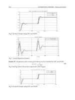
Equation (12.30), the MIRR for project A is
The calculation of MIRR for project A is illustrated in Figure 12.20.

Likewise, the MIRR for project B is
$,
.
$, . $, . $, .
$, . $ , .
$, . $, . $, .
$, . $
25 000
110
3 000 1 10 5 000 1 10 7 000 1 10
9 000 1 10 11 000 1 10
1
3 000 1 4641 5 000 1 331 7 000 1 21
9 000 1 10 11
0
432
10
5
()
=
()
+
()
+
()
+
()
+
()
+

()
=
()
+
()
+
()
+
()
+
MIRR
B
,,
$, . $, . $, . $, $ ,
000
1
4 392 30 6 655 00 8 470 00 9 900 11 000
1
5
5
+
()
=
++++
+
()
MIRR
MIRR
B
B

SS
tnt
t
tnt
nt
B
n
O
k
Rk
MIRR
=Æ =Æ
-
+
()
=
+
()
+
()
11
1
1
1
$,
.
$, . $, . $, .
$, . $, .
$, $, $, $, $,
$,

$,
25 000
110
10 000 1 10 8 000 1 10 6 000 1 10
5 000 1 10 4 000 1 10
1
14 641 10 648 7 260 5 500 4 000
1
25 000
42 049
1
0
432
10
5
5
()
=
()
+
()
+
()
+
()
+
()
+
()
=

++++
+
()
=
+
MIRR
MIRR
A
A
MIRRMIRR
MIRR
MIRR
MIRR
A
A
A
A
()
+
()
==
+=
=
5
5
1
42 049
25 000
1 68196
1 1 1096

0 1096
$,
,
.
.
. , or 10.96%
SS
tnt
t
tnt
nt
A
n
O
k
Rk
MIRR
=Æ =Æ
-
+
()
=
+
()
+
()
11
1
1
1

Methods for Evaluating Capital Investment Projects 535
The calculation of MIRR for project B is illustrated in Figure 12.21.
Based on the foregoing calculations, project A will be preferred to
project B because MIRR
A
> MIRR
B
.To reiterate, although the NPV method
should be preferred to both the IRR and MIRR methods, the MIRR method
is superior to the IRR method for two reasons. Unlike the IRR method, the
$,
$, .
$, .
$,
.
.
.,
25 000
40 417 30
1
1
40 417 30
25 000
1 616692
1 1 1008
0 1008
5
5
=
+

()
+
()
==
+=
=
MIRR
MIRR
MIRR
MIRR
B
B
B
A
or 10.08%
536 Capital Budgeting
+
0
1234 t
MIRR
B
=10.08%
$3,000 $5,000 $7,000 $9,000 $11,000
Ϫ
5
Ϫ$5,000
$11,000.00
9,900.00
8,470.00
6,655.00

4,392.30
$40,417.30 = TV
$25,000
$25,000
NPV =0
NPV of TV
͖
k =10%
–
FIGURE 12.21 Modified internal rate of return for project B.
+
0
1234 t
MIRR
A
=10.96%
$10,000 $8,000 $6,000 $5,000 $4,000
Ϫ
5
Ϫ$5,000
$4,000
5,500
7,260
10,648
14,641
$42,049 = TV
$25,000
$25,000
NPV= 0
NPV of TV

͖
k =10%
–
FIGURE 12.20 Modified internal rate of return for project A.