Managerial economics theory and practice phần 9 potx

Chapter 1) referred to this common understanding of the problem as “con-
ventional wisdom.” Shelling illustrated the concept of focal-point equilib-
ria with the following “abstract puzzles.”
1. A coin is flipped and two players are instructed to call “heads” or
“tails.” If both players call “heads,” or both call “tails,” then both win a prize.
If one player calls “heads” and the other calls “tails,” then neither wins a
prize.
2. A player is asked to circle one of the following six numbers: 7, 100,
13, 261, 99, and 555. If all of the players circle the same number, then each
wins a prize; otherwise no one wins anything.
focal-point equilibrium 587
3. A player is asked to put a check mark in one sixteen squares, arranged
as shown. If all the players check the same square, each wins a prize;
otherwise no one wins anything.
4. Two players are told to meet somewhere in New York City, but neither
player has been told where the meeting is to occur. Neither player has ever
been placed in this situation before, and the two are not permitted to com-
municate with each other. Each player must guess the other’s probable
location.
5. In the preceding scenario each player is told the date, but not the time,
of the meeting. Each player must guess the exact time that the meeting is
to take place.
6. A player is told to write down a positive number. If all players write
the same number, each player wins a prize; otherwise no one wins anything.
7. A player is told to name an amount of money. If all players name the
same amount, each wins that amount.
8. A player is asked to divide $100 into two piles labeled pile A and
pile B. Another player is asked to do the same. If the amounts in all
four piles coincide, player each receives $100, otherwise, neither player wins
anything.
9. The results of a first ballot in an election were tabulated as follows:

Smith 19 votes
Jones 28 votes
Brown 15 votes
Robinson 29 votes
White 9 votes
A second ballot is to be taken. A player is asked to predict which can-
didate will receive a majority of votes on the second ballot. The player has
no interest in the outcome of the second ballot. The player who correctly
predicts the candidate receiving the majority of votes will win a prize, and
everyone knows that a correct prediction is in everyone’s best interest. If
the player incorrectly predicts the “winner” of the second ballot, he or she
will win nothing.
In each of these nine scenarios there are multiple Nash equilibria.
Schelling found, however, that in an “unscientific sample of respondents,”
people tended to focus (i.e., to use focal points) on just a few such equilib-
ria. Schelling found, for example, that 86% of the respondents chose
“heads” in problem 1. In problem 2 the first three numbers received 90%
of the votes, with the number 7 leading the number 100 by a slight margin
and the number 13 in third place. In problem 4, an absolute majority of the
respondents, who were sampled in New Haven, Connecticut, proposed
meeting at the information booth in Grand Central Station, and virtually
all of them agreed to meet at 12 noon. In problem 6, two-fifths of all respon-
dents chose the number 1. In problem 7, 29% of the respondents chose $1
million, and only 7 percent chose cash amounts that were not multiples of
10. In problem 8, 88% of the respondents put $50 into each pile. Finally, in
problem 9, 91% of the respondents chose Robinson.
Schelling also found that the respondents chose focal points even when
these choices where not in their best interest. For example, consider the fol-
lowing variation of problem 1. Players A and B are asked to call “heads”
or “tails.” The players are not permitted to communicate with each other.

If both players call “heads,” player A gets $3 and player B gets $2. If both
players call “tails,” then player A gets $2 and player B gets $3. Again, if one
player calls “heads” and the other calls “tails,” neither player wins a prize.
In this scenario Schelling found that 73% of respondents chose “heads”
when given the role of player A. More surprising is that 68% of respon-
dents in the role of player B still chose “heads” in spite of the bias against
player B. The reader should verify that if both players attempt to win $3,
neither one will win anything.
The economic significance of focal-point equilibria becomes readily
apparent when we consider cooperative, non-zero-sum, simultaneous-
move, infinitely repeated games. Where explicit collusive agreements are
588 introduction to game theory
prohibited, the existence of focal-point equilibria suggests that tacit collu-
sion, coupled with the policing mechanism of trigger strategies, may be pos-
sible. A fuller discussion of these, and other related matters, is deferred to
the next section.
MULTISTAGE GAMES
The final scenario we will consider in this brief introduction to game
theory is that of the multistage game. Multistage games differ from the
games considered earlier in that play is sequential, rather than simultane-
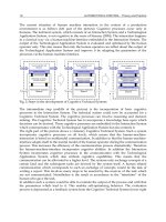
ous. Figure 13.12, which is an example of an extensive-form game, summa-
rizes the players, the information available to each player at each stage, the
order of the moves, and the payoffs from alternative strategies of a multi-
stage game.
Definition: An extensive-form game is a representation of a multistage
game that summarizes the players, the stages of the game, the information
available to each player at each stage, player strategies, the order of the
moves, and the payoffs from alternative strategies.
The extensive-form game depicted in Figure 13.12 has 2 players: player
A and player B. The boxes in the figure are called decision nodes. Inside

each box is the name of the player who is to move at that decision node.
At each decision node the designated player must decide on a strategy,
which is represented by a branch, which represents a possible move by a
player.The arrow indicates the direction of the move.The collection of deci-
sion nodes and branches is called a game tree. The first decision node is
called the root of the game tree. In the game depicted in Figure 13.12, player
A moves first. Player A’s move represents the first stage of the game. Player
A, who is at the root of the game tree, must decide whether to adopt a Yes
or a No strategy. After player A has decided on a strategy, player B must
multistage games 589
Player A
Player B
Player B
Yes
No
Yes
Yes
No
No
(15, 20)
(5, 5)
(0, 0)
(10, 25)
Pa
y
offs: (Pla
y
er A, Pla
y
er B)

FIGURE 13.12 Extensive-form game.
decide how to respond in the second stage of the game. For example, if
player A’s strategy is Yes, then player B must decide whether to respond
with a Yes or a No.
At the end of each arrow are small circles called terminal nodes.The
game ends at the terminal nodes. To the right of the terminal notes are the
payoffs. In Figure 13.12, the first entry in parenthses is the payoff to player
A and the second entry is the payoff to player B. If player B adopts a Yes
strategy, the payoff for player A is 15 and the payoff for player B is 20. In
summary, an extensive-form game is made up of a game tree, terminal
nodes, and payoffs.
As with simultaneous-move games, the eventual payoffs depend on the
strategies adopted by each player. Unlike simultaneous-move games, in
multistage games the players move sequentially. In the game depicted in
Figure 13.12, player A moves without prior knowledge of player B’s
intended response. player B’s move, on the other hand, is conditional on
the move of player A. In other words, while player B moves with the knowl-
edge of player A’s move, player A can only anticipate how player B will
react. The ideal strategy profile for player A is {Yes, Yes}, which yields
payoffs of (15, 20). For player B, the ideal strategy profile is {No, No}, which
yields payoffs of (10, 25).The challenge confronting player B is to get player
A to say No on the first move. As we will see, the solution is for player B
to convince player A that regardless of what player A says, player B will
say No. To see this, consider the following scenario.
Suppose that player B announces that he or she has adopted the fol-
lowing strategy: if player A says Yes, then player B will say No; if player A
says No, player B will also say No
. With the first strategy profile {Yes, No}
the payoffs are (5, 5). With the second strategy profile the payoffs are (10,
25). In this case, it would be in player A’s best interest to say No. Of course,

the choice of strategies is a “no brainer” if player A believes that player B
will follow through on his or her “threat.” player A’s first move will be No
because the payoff to player A from a {No, No} strategy is greater than from
a {Yes, No} strategy. In fact, the strategy profile {No, No} is a Nash equilib-
rium. Why? If player B’s threat to always say No is credible, then player A
cannot improve his or her payoff by changing strategies.
As the reader may have already surmised, the final outcome of this game
depends crucially on whether player A believes that player B’s threat to
always say No is credible. Is there a reason to believe that this is so? Prob-
ably not. To see this, assume again that the optimal strategy profile for
player A is {Yes, Yes}, which yields the payoff (15, 20). If player A says Yes,
the payoff to player B from saying No is 5, but the payoff for saying Yes is
20. Thus, if player B is rational, the threat to say No lacks credibility and
the resulting strategy profile is {Yes, Yes}.
Note that strategy profile {Yes, Yes} is also a Nash equilibrium. Neither
player can improve his or her payoff by switching strategies. In particular,
590 introduction to game theory
if player B’s strategy was to say Yes if player A says Yes and say No if player
A says No, then player A’s payoff is 15 by saying Yes and 10 by saying No.
Clearly, player A’s best strategy, given player B’s move, is to say Yes.
We now have two Nash equilibria. Which one is the more reasonable?
It is the Nash equilibrium corresponding to the strategy profile {Yes, Yes}
because player B has no incentive to carry through with the threat to say
No. The Nash equilibrium corresponding to the strategy profile {Yes, Yes}
is referred to as a subgame perfect equilibrium because no player is able to
improve on his or her payoff at any stage (decision node) of the game by
switching strategies. In a subgame perfect equilibrium, each player chooses
at each stage of the game an optimal move that will ultimately result in
optimal solution for the entire game. Moreover, each player believes that
all the other players will behave in the same way.

Definition: A strategy profile is a subgame perfect equilibrium if it is a
Nash equilibrium and allows no player to improve on his or her payoff by
switching strategies at any stage of a dynamic game.
The idea of a subgame perfect equilibrium may be attributed to Rein-
hard Selten (1975). Selten formalized the idea that a Nash equilibrium with
incredible threats is a poor predictor of human behavior by introducing the
concept of the subgame. In a game with perfect information, a subgame is
any subset of branches and decision nodes of the original multistage game
that constitutes a game in itself. The unique initial node of a subgame is
called a subroot of the larger multistage game. Selten’s essential contribu-
tion is that once a player begins to play a subgame, that player will con-
tinue to play the subgame until the end of the game. That is, once a player
begins a subgame, the player will not exit the subgame in search of an alter-
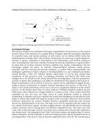
native solution. To see this, consider Figure 13.13, which recreates Figure
13.12.
multistage games 591
Payoffs: (Player A, Player B)
Player A
Player B
Player B
Yes
No
Yes
Yes
No
No
(15, 20)
(5, 5)
(0, 0)
(10, 25)

T
1
S
2
S
3
S
1
T
2
T
3
T
4
FIGURE 13.13 A subgame.
Figure 13.13 is a multistage game consisting of two subgames. The mul-
tistage game itself begins at the initial node, S
1
. The two subgames begin at
subroots S
2
and S
3
. The subgame that begins at subroot S
2
, which is high-
lighted by the dashed, rounded rectangle, has two terminal nodes, T
1
and
T

2
, with payoffs of (15, 20) and (5, 5), respectively. In games with perfect
information, every decision node is the subroot of a larger game. A player
who begins a subgame is common knowledge to all the other players. The
student should verify that this subgame has a unique Nash equilibrium. At
this Nash equilibrium player B says Yes. The reader should also verify that
the subgame with subroot S
3
also has a unique Nash equilibrium.
As we have seen, the final outcome of the multistage game depicted in
Figure 13.12 depends on whether player A believes that player B’s threat
to say No is credible. If player B is rational, the threat to say No lacks cred-
ibility and the resulting strategy profile is {Yes, Yes}. Thus, the nonoptimal-
ity of the strategy profile {No, No} makes player B’s threat incredible. Thus,
this strategy profile is eliminated by the requirement that Nash equilibrium
strategies remain when applied to any subgame. A Nash equilibrium with
this property is called a subgame perfect equilibrium. The Nash equilibrium
corresponding to the strategy profile {Yes, Yes} is referred to as a subgame
perfect equilibrium because no player is able to improve on his or her
payoff at any stage (decision node) of the game by switching strategies. As
we will soon see, the concept of a subgame perfect equilibrium is essential
element of the backward induction solution algorithm.
EXAMPLE: SOFTWARE GAME
As we have already seen, one of the problems with multistage games is
the selection of an optimal strategy profile in the presence of multiple Nash
equilibria. This issue will be addressed in later sections. For now, consider
the following example of a subgame perfect equilibrium, which comes
directly from Bierman and Fernandez (1998, Chapter 6).
Macrosoft Corporation is a computer software company that is planning
to introduce a new computer game into the market. Macrosoft’s manage-

ment is considering two marketing approaches. The first approach involves
a “Madison Avenue” type of advertising campaign, while the second
approach emphasizes word of mouth. Bierman and Fernandez described
the first approach as “slick” and the second approach as “simple.”
The timing involved in both approaches is all-important in this example.
Although expensive, the “slick” approach will result in a high volume of
sales in the first year, while sales in the second year are expected to decline
dramatically as the market becomes saturated. The inexpensive “simple”
approach, on the other hand, is expected to result in relatively low sales
volume in the first year, but much higher sales volume in the second year
as “word gets around.” Regardless of the promotional campaign adopted,
592 introduction to game theory
no significant sales are anticipated after the second year. Macrosoft’s net
profits from both campaigns are summarized in Table 13.1.
The data presented in Table 13.1 suggest that Macrosoft should adopt
the inexpensive “simple” approach because of the resulting larger total
net profits. The problem for Macrosoft, however, is the threat of a “legal
clone,” that is, a competing computer game manufactured by another firm,
Microcorp, that is, to all outward appearances, a close substitute for origi-
nal. The difference between the two computer games is in the underlying
programming code, which is sufficiently different to keep the “copycat” firm
from being successfully sued for copyright infringement. In this example,
Microcorp is able to clone Macrosoft’s computer game within a year at a
cost of $300,000. If Microcorp decides to produce the clone and enter the
market, the two firms will split the market for the computer game in the
second year. The payoffs to both companies in years 1 and 2 are summa-
rized in Tables 13.2 and 13.3.
Given the information provided in Tables 13.2 and 13.3 what is the
optimal marketing strategy for each player, Macrosoft and Microcorp?
Since the decisions of both companies are interdependent and sequential

the problem may be represented as the extensive-form game in Figure
13.14.
It should be obvious from Figure 13.14 that Macrosoft moves first and
has just one decision node. The choices facing Macrosoft consist of “slick”
multistage games 593
TABLE 13.1 Macrosoft’s Profits if Microcorp Does Not
Enter the Market
Slick Simple
Gross profit in year 1 $900,000 $200,000
Gross profit in year 2 $100,000 $800,000
Total gross profit $1,000,000 $1,000,000
Advertising cost -$570,000 -$200,000
Total net profit $430,000 $800,000
TABLE 13.2 Macrosoft’s Profits if Microcorp Enters
the Market
Slick Simple
Gross profit in year 1 $900,000 $200,000
Gross profit in year 2 $50,000 $400,000
Total gross profit $950,000 $600,000
Advertising cost -$570,000 -$200,000
Total net profit $380,000 $400,000
and “simple.” Microcorp, on the other hand, has two decision nodes. Micro-
corp’s strategy is conditional on Macrosoft’s decision of a promotional
campaign. For example, if Macrosoft decides upon a “slick” campaign,
Microcorp might decide to “stay out” of the market. On the other hand, if
Macrosoft decides on a “simple” campaign, Microcorp might decide that its
best move is to “enter” the market.This strategy profile for Microcorp might
be written {Stay out, Enter}. As the reader will readily verify, there are four
possible strategy profiles available to Microcorp. These strategy profiles
represent Microcorp’s contingency plans. Which strategy is adopted will

depend on Macrosoft’s actions. Since different strategies will often result in
the same sequence of moves, it is important not to confuse strategies with
actual moves.
NASH EQUILIBRIUM AND BACKWARD
INDUCTION
At this point we naturally are interested in the strategic choices of each
player.As we will soon see, finding an optimal solution for multistage games
594 introduction to game theory
TABLE 13.3 Microcorp’s Profits after Entering the
Market
Slick Simple
Gross profit in year 1 $0 $0
Gross profit in year 2 $50,000 $400,000
Total gross profit $50,000 $400,000
Cloning cost -$300,000 -$300,000
Total net profit $250,000 $100,000
Payoffs: (Macrosoft, Microcorp)
Macrosoft
Microcorp
Microcorp
Slick
Simple
Enter
Enter
Stay out
Stay out
($380,000,
Ϫ
$250,000)
($430,000, $0)

($400,000, $100,000)
($800,000, $0)
FIGURE 13.14 The software game.
is not nearly as simple as it might seem at first glance. This is because
multistage noncooperative games are often plagued with multiple Nash
equilibria.A solution concept is a methodology for finding solutions to mul-
tistage games. There is no universally accepted solution concept that can be
applied to every game. Bierman and Fernandez (1998, Chapter 6) have pro-
posed the backward induction concept for finding optimal solutions to mul-
tistage games involving multiple Nash equilibria. The backward induction
method is sometimes referred to as the fold-back method.
Definition: Backward induction is a methodology for finding optimal
solutions to multistage games involving multiple Nash equilibria.
The solution concept of backward induction will be applied to the mul-
tistage game depicted in Figure 13.14, which assumes that Macrosoft and
Microcorp have perfect information. Perfect information consists of player
awareness of his or her position on the game tree whenever it is time to
move. Before discussing the backward induction methodology, consider
again the payoffs (in $000’s) in Figure 13.14, which is summarized as the
normal-form game in Figure 13.15.
Now consider the noncooperative solution to the game depicted in
Figure 13.15. The reader should verify that a Nash equilibrium to this game
is the strategy profile {Enter, Simple}. It will be recalled that in a Nash equi-
librium, each player adopts a strategy it believes is the best response to the
other player’s strategy and neither player’s payoff can be improved by
changing strategies.
The limitation of a Nash equilibrium as a solution concept is that chang-
ing the strategy of any single player may result in a new Nash equilibrium,
which may be not be an optimal solution. To see this, consider Figure 13.16,
which is the strategic form of the multistage game in Figure 13.14.

Strategic-form games illustrate the payoffs to each player from every pos-
sible strategy profile. Macrosoft, for example, may adopt one of two pro-
motional campaigns—Slick or Simple. Microcorp, on the other hand, may
adopt one of four strategic responses: (Enter, Enter), (Enter, Stay out), (Stay
out, Enter), or (Stay out, Stay out).
Definition: The strategic form of a game summarizes the payoffs to each
player arising from every possible strategy profile.
multistage games 595
Macrosoft
Slick Simple
Microcorp
Enter ( $
Ϫ
250,000, $380,000) ($100,000, $400,000)
Stay out ($0, $430,000) ($0, $800,000)
Payoffs: (Microcorp, Macrosoft)
FIGURE 13.15 Payoff matrix for a two-player, simultaneous-move game.
The cells in Figure 13.16 summarize the payoffs from all possible strate-
gic combinations. For example, suppose that Microcorp decides to “enter”
regardless of the promotional campaign adopted by Macrosoft. In this case,
Macrosoft will select a “simple” campaign, which is the Nash equilibrium
of the normal-form game illustrated in Figure 13.15. The strategy profile for
this game may be written {Simple,(Enter, Enter)}. On the other hand, if
Macrosoft adopts a “slick” strategy, Microcorp can do no better than to
adopt the strategy (Stay out, Enter). The strategy profile for this game
may be written {Slick,(Stay out, Enter)}. This is a Nash equilibrium for the
strategic-form game in Figure 13.16 but is not a Nash equilibrium for the
normal-form game in Figure 13.15!
Finding an optimal solution to a multistage game using the backward
induction methodology involves five steps:

1. Start at the terminal nodes. Trace each node to its immediate prede-
cessor node. The decisions at each node may be described as “basic,”
“trivial,” or “complex.” Basic decision nodes have branches that lead to
exactly one terminal node. Basic decision nodes are trivial if they have only
one branch. A decision node is complex if it is not basic, that is, if at least
one branch leads to more than one terminal node. If a trivial decision node
is reached, continue to move up the decision tree until a complex or a non-
trivial decision node is reached.
2. Determine the optimal move at each basic decision node reached in
step 1. A move is optimal if it leads to the highest payoff.
3. Disregard all nonoptimal branches from decision nodes reached in
step 2. With the nonoptimal branches disregarded, these decision nodes
become trivial (i.e., they now have only one branch). The resulting game
tree is simpler than the original game tree.
4. If the root of the game tree has been reached, then stop. If not, repeat
steps 1–3. Continue in this manner until the root of the tree has been
reached.
596 introduction to game theory
Macrosoft
Slick Simple
(Enter, Enter)
(
$
Ϫ
250,000, $380,000) ($100,000, $400,000)
Microcorp
(Enter, Stay out) $250,000, $380,000) ($0, 800,000
)
(Stay out, Enter) ($0, $430,000) ($100,000
$400,000

(Stay out, Stay out) ($0, $430,000) ($0,
$800,000
(
Ϫ
Payoffs: (Microcorp, Macrosoft)
FIGURE 13.16 Payoff matrix for a strategic-form game.
5. After the root of the game tree has been reached, collect the optimal
decisions at each player’s decision nodes. This collection of decisions com-
prises the players’ optimal strategies.
The backward induction solution concept will now be applied to the mul-
tistage game depicted in Figure 13.14. From each terminal node, move to
the two Microcorp decision nodes. Each of these decision nodes is basic,
since the branches lead to exactly one terminal node. If Macrosoft chooses
a “slick” campaign, the optimal move for Microcorp is to stay out, since the
payoff is $0 compared with a payoff of -$250,000 by entering. The “enter”
branch should be disregarded in future moves. If Macrosoft chooses a
“simple” campaign, the optimal move for Microcorp is to enter, since the
payoff is $100,000 compared with a payoff of $0 by staying out. This “stay
out” branch should be disregarded in future moves.The resulting extensive-
form game is illustrated in Figure 13.17.
An examination of Figure 13.17 will reveal that the optimal strategy for
Microcorp is (Stay out, Enter). The final optimal strategy profile is {Slick,
(Stay out, Enter)}, which yields payoffs of $430,000 for Macrosoft and $0 for
Microcorp. The reader should note that the choice of this Nash equilibrium
($0, $430,000) from Figure 13.16 differs from the Nash equilibrium
($100,000, $400,000) in Figure 13.12.The implication of the backward induc-
tion method is straightforward. By taking Microcorp’s entry decision into
account, Macrosoft avoided making a strategy decision that would have cost
it $30,000.
Problem 13.8. Consider, again, the strategy for the software game sum-

marized in Figure 13.17. Suppose that the cost of cloning Macrosoft’s com-
puter game is $10,000 instead of $300,000.
multistage games 597
Macrosoft
Microcorp
Microcorp
Slick
Simple
Enter
Enter
Stay out
Stay out
($380,000, Ϫ$250,000)
($430,000, $0)
($400,000, $100,000)
($800,000, $0)
Pa
y
offs: (Macrosoft, Microcorp)
FIGURE 13.17 Using backward induction to find a Nash equilibrium.
a. Diagram the new extensive-form for this multistage game.
b. Use the backward induction solution concept to determine the new
optimal strategy profile for this game. Illustrate your answer.
Solution
a. Microcorp’s profits at the lower cost of cloning Macrosoft’s computer
game and entering the market are presented in Table 13.4.
Assuming that Macrosoft’s net profits remain unchanged, the extensive
form of this game is as shown in Figure 13.18.
b. Using the backward induction solution methodology, from each termi-
nal node move to Microcorp’s two decision nodes. Each of these deci-

sion nodes is basic. If Macrosoft chooses a Slick campaign, the optimal
move for Microcorp is to Enter, since the payoff is $40,000 compared
with a payoff of $0 by staying out. The Stay out branch should be disre-
garded in future moves. If Macrosoft chooses a Simple campaign, the
optimal move for Microcorp is to Enter, since the payoff is $390,000 com-
pared with a payoff of $0 if it adopts a Stay out strategy. The Stay out
branch should be disregarded in future moves. In the resulting extensive-
form game, diagrammed in Figure 13.19, we see that the optimal strat-
egy for Microcorp is (Enter, Enter). The final optimal strategy profile is
{Simple,(Enter, Enter)}, which yields payoffs of $400,000 for Macrosoft
and $390,000 for Microcorp.
Problem 13.9. Suppose that in Problem 13.8 the cost of cloning
Macrosoft’s computer game is $500,000 instead of $300,000.
a. Diagram the new extensive-form for this multistage game.
b. Use the backward induction solution concept to determine the new
optimal strategy profile for this game. Illustrate your answer.
Solution
a. Microcorp’s profits at the higher cost of cloning Macrosoft’s computer
game and entering the market are presented in Table 13.5.
The extensive form of this game, assuming that Macrosoft’s net profits
remain unchanged, is diagrammed in Figure 13.20.
598 introduction to game theory
TABLE 13.4 Microcorp’s Profits after Entering the
Market
Slick Simple
Gross profit in year 1 $0 $0
Gross profit in year 2 $50,000 $400,000
Total gross profit $50,000 $400,000
Cloning cost -$10,000 -$10,000
Total net profit $40,000 $390,000

multistage games 599
Payoffs: (Macrosoft, Microcorp)
Macrosoft
Microcorp
Microcorp
Slick
Simple
Enter
Enter
Stay out
Stay out
($380,000, $40,000)
($430,000, $0)
($400,000, $390,000)
($800,000, $0)
FIGURE 13.18 Game tree for problem 13.8.
Pa
y
offs: (Macrosoft, Microcorp)
Macrosoft
Microcorp
Microcorp
Slick
Simple
Enter
Enter
Stay out
Stay out
($380,000, $40,000)
($430,000, $0)

($400,000, $390,000)
($800,000, $0)
FIGURE 13.19 Solution to problem 13.8 using backward induction.
TABLE 13.5 Microcorp’s Profits after Entering the
Market
Slick Simple
Gross profit in year 1 $0 $0
Gross profit in year 2 $50,000 $400,000
Total gross profit $50,000 $400,000
Cloning cost $500,000 $500,000
Total net profit -$450,000 -$100,000
b. Using the backward induction solution concept, from each terminal node
move to Microcorp’s two decision nodes. Each of these decision nodes
is basic. If Macrosoft chooses a “slick” campaign, the optimal move for
Microcorp is to stay out, since the payoff is $0 compared with a payoff
of -$450,000 by entering. The “enter” branch should be disregarded
in future moves. If Macrosoft chooses a “simple” campaign, again
the optimal move for Microcorp is to stay out, since the payoff is $0
compared with a payoff of -$100,000. The “enter” branch should be
disregarded in future moves. In the resulting extensive-form game,
diagrammed in Figure 13.21, we see that the optimal strategy for Micro-
corp is (Stay out, Stay out). The final optimal strategy profile is {Simple,
(Stay out, Stay out)}, which yields payoffs of $800,000 for Macrosoft and
$0 for Microcorp.
600 introduction to game theory
Macrosoft
Microcorp
Microcorp
Slick
Simple

Enter
Enter
Stay out
Stay out
($380,000, –$450,000)
($430,000, $0)
($400,000, –$100,000)
($800,000, $0)
Pa
y
offs: (Macrosoft, Microcorp)
FIGURE 13.20 Game tree for problem 13.9.
Macrosoft
Microcorp
Microcorp
Slick
Simple
Enter
Enter
Stay out
Stay out
($380,000, –$450,000)
($430,000, $0)
($400,000, –$100,000)
($800,000, $0)
(Payoffs: Macrosoft, Microcorp)
FIGURE 13.21 Solution to problem 13.9 using backward induction.
Problem 13.10. Consider again the multistage game in Figure 13.12. Use
the backward induction solution concept to determine the optimal strategy
profile for this game. Illustrate your answer.

Solution. Using the backward induction solution concept, from each ter-
minal node move to the two Microcorp decision nodes. Each of these deci-
sion nodes is basic. If player A says “yes,” the optimal move for player B is
to say “yes,” since the payoff is $20 compared with $5 by saying “no.” Thus,
the “no” branch should be disregarded in future moves. If player A says
“no,” the optimal move for player B is to say “no” since the payoff is $25
compared with $0 by saying “yes.” The “yes” branch should be disregarded
in future moves. In the resulting extensive-form game, diagrammed in
Figure 13.22, we see that the optimal strategy for player B is (Yes, No). The
final optimal strategy profile is {Yes,(Yes, No)}, which yields payoffs of 15
for player A and 20 for player B.The student is encouraged to compare this
result with the earlier discussion of the selection of Nash equilibria with
credible threats.
BARGAINING
In Chapter 8, perfectly competitive markets were characterized by large
numbers of buyers and sellers. Firms in perfectly competitive industries
were described as “price takers” because of their inability in influence the
market price through individual production decisions. Consumers in such
markets may similarly be described as price takers because they are indi-
vidually incapable of extracting discounts or better terms from sellers. Since
neither the buyer nor seller has “market power,” the theoretical ability to
“haggle” over the terms of the sale, or product content, is nonexistent. In
bargaining 601
Payoffs: (Player A, Player B)
Player A
Player B
Player B
Yes
No
Yes

Yes
No
No
(15, 20)
(5, 5)
(0, 0)
(10, 25)
FIGURE 13.22 Solution to problem 13.10 using backward induction.
the case of a monopolist selling to many small buyers, which was also dis-
cussed in Chapter 8, it was assumed that firms set the selling price of the
product, and buyers, having no place else to go, accept that price without
question. Even when of a neither the buyer or the seller may be thought of
as a “price taker,” such as the case monopsonist selling to an oligopolist,
economists have had little to say about the possibility of negotiating, or
“bargaining” over the contract terms.
Yet, bargaining is a fact of life. Whether bargaining with the boss for an
increase in wages and benefits or haggling over the price of a new car, such
interactions between buyer and seller are commonplace. In many instances,
contract negotiations between producer and supplier, contractor and sub-
contractor, wholesaler and distributor, retailer and wholesaler, and so on,
are the norm, rather than the exception. As an exercise, the reader is asked
to consider why market power and the ability to bargain with product sup-
pliers allow large retail outlets, such as Home Depot, Sports Authority, or
Costco, to offer prices that are generally lower than those featured at the
local hardware store, sporting goods store, or other retailer. Even in markets
characterized by many buyers and sellers, it is often possible to find
“pockets” of local monopoly or monopsony power that permits limited bar-
gaining over contract terms to take place. Game theory is a useful tool for
analyzing and understanding the dynamics of the bargaining process.
BARGAINING WITHOUT IMPATIENCE

We will begin our discussion of the bargaining process by considering
the following scenario. Suppose that Andrew wishes to purchase an annual
service contract from Adam. It is known by both parties that Andrew is
willing to pay up to $100 for the service contract and that Adam will not
accept any offer below $50. The maximum price that Andrew is willing to
pay is called the buyer’s reservation price and the minimum price that Adam
is willing to accept is called the seller’s reservation price. If Andrew and
Adam can come to an agreement, the gain to both will add up to the dif-
ference between the buyer’s and the seller’s reservation prices, which in this
case is $50.
Negotiations between Andrew and Adam may be modeled as the
extensive-form game illustrated in Figure 13.23. We will assume for sim-
plicity that negotiations involve only two offers and that Andrew makes
the first offer, which is denoted as P
1
. This is indicated as the first branch of
the decision tree. After Andrew has made the offer, Adam can either accept
or reject it. If Adam accepts the offer, the bargaining process is completed
and the payoffs for Andrew and Adam are (100 - P
1
, P
1
- 50), respectively.
For example, if Adam accepts Andrew’s offer of, say, $80, then Andrew’s
gain from trade is $20 and Adam’s gain from trade is $30, which sum to the
difference between the respective parties’ reservation prices. If Adam
602 introduction to game theory
rejects Andrew’s offer, Adam can come back with a counteroffer, which is
denoted as P
2

. If Andrew accepts Adam’s counteroffer, the payoffs to
Andrew and Adam are (100 - P
2
, P
2
- 50), respectively. If, on the other
hand, Andrew rejects Adam’s counteroffer, this game comes to an end and
no agreement is reached, in which case the payoffs are (0, 0).
Earlier we discussed the procedure of backward induction for finding
solution values to multistage games with multiple equilibria. Applying this
approach to the present bargaining game, it is easy to see that as long as
Adam’s counteroffer is not greater than $100, Andrew will accept. The
reason for this is that Andrew cannot do any better than to accept an offer
that does not exceed $100. Moving up the game tree to another node, it is
equally apparent that Adam will reject any offer by Andrew that is less than
$100. Moreover, accepting the offer ignores the fact that Adam has the
ability to make a more advantageous (to him) counteroffer in the next
round of negotiations. What all this means is that no matter what Andrew’s
initial offer was, he will end up paying Adam $100. In other words, as long
as Adam has the ability to make a counteroffer, Adam will never accept
Andrew’s offer as final! Thus, in the two rounds of negotiation in this game,
since Adam has the last move, then Adam “holds all the cards.” The ability
of Adam to dictate the final terms of the negotiations is referred to as the
last-mover’s advantage. Andrew might just as well save his breath and offer
Adam $100 at the outset of the bargaining process.
As the scenario illustrates, the final outcome of this class of bargaining
processes depends crucially on who makes the first offer, and on the number
of rounds of offers.The reader can verify, for instance, that if Andrew makes
the first offer, and there are an odd number of rounds of negotiations,
Andrew has the last-mover’s advantage, in which case Andrew will be able

to extract the entire surplus of $50. If such is the case, it will be in both
parties’ best interest for Adam to accept Andrew’s initial offer of $50,
thereby saving both individuals the time, effort, and aggravation of an
bargaining 603
Pa
y
offs: (Andrew, Adam)
Andrew
Adam Andrew
Adam
Accept
Accept
Reject
Reject
Offer
Counteroffer
(0, 0)
(100ϪP
2
, P
2
Ϫ50)
(100ϪP
1
, P
1
Ϫ50)
FIGURE 13.23 Bargaining without impatience.
extended bargaining process. Similarly, if Adam has the first move and there
are an even number of rounds of negotiations, it will in both parties’ inter-

est for Andrew to accept Adam’s initial offer $100. In this case, Adam will
extract the entire surplus of $50.
BARGAINING WITH SYMMETRIC IMPATIENCE
If negotiations of the type just described were that simple, bargaining
would never take place. Of course, bargaining is a fact of life, so something
must be missing. In this section we will make the underlying conditions of
the bargaining process somewhat more realistic by assuming that there are
multiple rounds of offers and counteroffers and costs associated with not
immediately reaching an agreement. In the terminology of capital bud-
geting, this section will introduce the time value of money by discounting
to the present future payoffs from negotiations.
In the example of bargaining without impatience, it was assumed that
there were only two rounds of bargaining. In fact, the bargaining process is
likely to involve multiple rounds of offer and counteroffer lasting days,
weeks, or months. Failure to reach an agreement immediately may impose
considerable costs on the bargainers. Consider, for example, the rather large
opportunity costs incurred by a person who discovers that his or her car has
been stolen. It is Saturday and the person needs to be able to drive to work
on Monday. Although the stolen car was old, and the person was planning
to buy another car anyway, the theft has the introduced a higher than usual
level of anxiety into the situation. Failure to quickly come to terms on the
purchase price of a replacement car may result not only in high psycho-
logical opportunity costs but in lost income, as well.
In this scenario, the buyer can take one of two possible approaches in
negotiations with the used-car salesman. On the one hand, the buyer can
withhold from the seller the details of his or her ill fortune and negotiate
with a “cool head.” Alternatively, the buyer may be unable, or unwilling, to
withhold knowledge of the theft, preferring to attempt to garner under-
standing and sympathy. As we will soon see, sympathy in the bargaining
process is not without cost: when one person’s gain is another’s loss, a buyer

seeking sympathy will be better off visiting a psychiatrist, not a used-car
salesman. To see this, let us consider the situation in which the buyer and
the seller enter into negotiations without any knowledge of the opportu-
nity costs that may be imposed on the other because of a failure to imme-
diately reach an agreement. This situation is equivalent to the situation of
the buyer who negotiates with the used-car salesperson with a “cool head.”
Suppose, once again, that Andrew wishes to purchase an annual service
contract from Adam, that Andrew is willing to pay up to $100 for the service
contract and that Adam will not accept any offer below $50. Instead of
only two negotiating rounds, however, suppose that there are 50 offer–
604 introduction to game theory
counteroffer rounds. Since neither Andrew nor Adam knows anything
about the other’s personal circumstances, let us further assume that any
delay in reaching an agreement reduces the gains from trade to both by 5%
per round.This assumption is equivalent to assuming that both players have
symmetric patience. We will assume that both players are aware of the cost
imposed on the other by failing to come to an agreement immediately.
With 50 rounds of negotiations, it is impractical to illustrate the bargaining
process as an extensive-form game. Nevertheless, it is still possible to use
backward induction to determine Andrew’s and Adam’s negotiating strate-
gies. Consider the information summarized in Table 13.6.
We know that since Andrew makes the first offer and there are an even
number of negotiating rounds, Adam has the last-mover’s advantage. Thus,
if negotiations drag on to the 50th round, Adam will sell the service con-
tract for $100 and extract the entire surplus of $50.Andrew,of course, knows
this. Andrew also knows that Adam will be indifferent between receiving
$100 in the 50th round and receiving the entire surplus of $50, or receiving
$97.50 in the 49th round because delays in reaching an agreement reduce
Adam’s gain by 5% per round. Thus, Adam will accept any offer from
Andrew of $97.50 or more in the 49th round, which results in a surplus of

$47.50, and reject any offer that is less than that. In capital budgeting ter-
minology, the time value of $97.50 in the 49th round for Adam is the same
as the time value of $100 in the 50th round. But this is not the end of the
game.
Adam also knows that delays in reaching an agreement will reduce
Andrew’s gain from trade by 5% per round. Thus, Andrew is indifferent
between receiving a surplus of $2.50 in the 49th round or receiving 5% less
($2.38) in the 48th round. Thus, Adam should offer to sell the service con-
tract for $97.62 in the 48th round, thereby receiving a surplus of $47.62.
bargaining 605
TABLE 13.6 Nash Equilibrium with Symmetric Impatience
Round Offer maker Offer price Adam’s surplus Andrew’s surplus
50 Seller $100.00 $50.00 $0.00
49 Buyer $97.50 $47.50 $2.50
48 Seller $97.62 $47.62 $2.38
47 Buyer $95.24 $45.24 $4.76
46 Seller $95.48 $45.48 $4.52
ӇӇ Ӈ Ӈ Ӈ
5 Buyer $76.78 $26.78 $23.22
4 Seller $77.94 $27.94 $22.06
3 Buyer $76.55 $26.55 $23.46
2 Seller $77.72 $27.72 $22.28
1 Buyer $76.33 $26.33 $23.67
Once again, Andrew knows that Adam is indifferent between a price of
$97.62 in the 48th round and $95.24 in the 47th round, which reduces
Adam’s surplus by 5%, to $45.24. Andrew’s surplus, on the other hand, will
increase to $4.76. Continuing in the same manner, the reader can verify
through the use of backward induction that Andrew’s best offer in the first
round is $76.33, which Adam should accept. Adam’s and Andrew’s gains
from trade are $26.33 and $23.67, respectively. The reader might suspect

that if this process is continued, eventually Andrew and Adam will evenly
divide the surplus; but as long as Adam moves last, he will enjoy an advan-
tage, however slight, over Andrew.
BARGAINING WITH ASYMMETRIC IMPATIENCE
Suppose that instead of maintaining an “even keel” the buyer reveals to
the used-car salesman the importance of quickly replacing the stolen car.
The used-car salesman will immediately recognize the higher opportunity
cost to the buyer from delaying a final agreement. To demonstrate the
impact that his knowledge has on the bargaining process, consider again the
negotiations between Andrews and Adam. We will continue to assume that
there are 50 rounds of negotiations, but that the opportunity cost to Andrew
from delaying an agreement reduces the gain from trade by 10% per round,
while the opportunity cost to Adam continues to be 5% per round. Pro-
ceeding as before, the information in Table 13.7 summarizes the gains from
trade to both Andrew and Adam that result from bargaining in the pres-
ence of asymmetric impatience (i.e., different opportunity costs for each
player).
Utilizing backward induction, the reader will readily verify from Table
13.7 that Andrew’s best first round offer is $83.10. This will result in a
606 introduction to game theory
TABLE 13.7 Nash Equilibrium with Asymmetric Impatience
Round Offer maker Offer price Adam’s surplus Andrew’s surplus
50 Seller $100.00 $50.00 $0.00
49 Buyer $97.50 $47.50 $2.50
48 Seller $97.75 $47.75 $2.25
47 Buyer $95.36 $45.36 $4.64
46 Seller $95.83 $45.83 $4.17
ӇӇ Ӈ Ӈ Ӈ
5 Buyer
4 Seller $84.91 $34.91 $15.09

3 Buyer $83.16 $33.16 $16.84
2 Seller $84.84 $34.84 $15.16
1 Buyer $83.10 $33.10 $16.90
surplus to Adam of $33.10, which is nearly twice the gain from trade enjoyed
by Andrew. The results presented in Table 13.7 demonstrate that the nego-
tiating party with the lowest opportunity cost has the clearest advantage in
the negotiating process.Within the context of the stolen car example, clearly
patience and secrecy are virtues. By “crying the blues” to the used-car sales-
man, the buyer placed himself or herself at a bargaining disadvantage.
Unless the buyer is dealing with a paragon of rectitude and virtue, looking
for sympathy from a rival during negotiations will clearly result in a disad-
vantageous division of the gains from trade.
If effect, impatience has been used as the discount rate for finding the
present value of gains from trade in bargaining. The greater the players’
impatience (the higher the discount rate), the less advantageous will be the
gains from bargaining. Ariel Rubinstein (1982) has demonstrated that in
this type of two-player bargaining game there exists a unique subgame
perfect equilibrium.Assume that, player A and player B are bargaining over
the division of a surplus and player B makes the first offer. Assume further
that there is no limit to the number of rounds of offer and counteroffer and
that both players accept offers when indifferent between accepting and
rejecting the offer. Denote player A’s discount rate as d
A
and Player B’s dis-
count rate as d
B
. A bargaining game has a unique subgame perfect equilib-
rium if in the first round player B offers player A
(13.15)
as a share of the surplus, where q

A
= 1 -d
A
and q
B
= 1 -d
B
. Player B’s share
of the surplus is
(13.16)
Problem 13.11. Andrew and Adam are bargaining over a surplus of
$50. Assume that there is no limit to the number of rounds of offer and
counteroffer, and that the discount rates for both players are d
A
= 0.05 and
d
B
= 0.05.
a. For a subgame perfect equilibrium to exist, what portion of the surplus
should Adam offer Andrew in the first round? What portion of the
surplus should Adam keep for himself?
b. Suppose that Adam’s discount rate is d
A
= 0.05 and Andrew’s discount
rate is d
B
= 0.10. What portion of the surplus should Adam offer Andrew
in the first round and what portion should he keep for himself?
Solution
a. q

A
= 1 -d
A
= 0.95; q
B
= 1 -d
B
= 0.95. Substituting these values into expres-
sion (13.15) we obtain
w
q
qq
B
A
AB
=
-
-
1
1
w
qq
qq
A
AB
AB
=
-
()
-

1
1
bargaining 607
The amount of the surplus that Adam should offer Andrew is
From equation (3.16) we obtain,
The share of the surplus that Adam should keep is, therefore,
Of course, the sum of the shared surpluses is $50. The student should
note that as the last mover,Adam earns slightly more of the surplus than
Andrew. The student is urged to compare these results with those found
in Table 13.6. For the same discount rates and 50 negotiating rounds
Adam received $26.33 and Andrew received $23.67.
b. q
A
= 1 -d
A
= 0.90; q
B
= 1 -d
B
= 0.95. Substituting these values into expres-
sion (13.15) we obtain
The amount of the surplus that Adam should offer Andrew is
The share of the surplus that Adam should keep for himself can be found
by first substituting the information provided into expression (13.16), or
The share of the surplus that Adam should keep is, therefore,
Once again, the sum of the shared surpluses is $50. The student should
note that, as the last mover, Adam retains more of the surplus then
Andrew.
CHAPTER REVIEW
Game theory is the study of the strategic behavior involving the interac-

tion of two or more individuals, teams, or firms, usually referred to as
w
B
=
()
=0 6897 50 34 48.$$.
w
q
qq
B
A
AB
=
-
-
=
-
-
()()
==
1
1
1090
1 0 90 0 95
010
0 145
0 6897
.

.

.
.
0 3103 50 15 52.$$.
()
=
w
wq
qq
A
AB
AB
=
-
()
-
=
()
-
()
-
()()
==
1
1
090 1 095
1 0 90 0 95
0 045
0 145
0 3103

.
.
.
w
B
$.$$.50 0 5128 50 25 64
()
=
()
=
w
q
qq
B
A
AB
=
-
-
=
-
()
-
()()
==
1
1
1095
1 0 95 0 95

005
0 0975
0 5128
.

.
.
.
w
A
$.$$.50 0 4872 50 24 3
6
()
=
()
=
w
wq
qq
A
AB
AB
=
-
()
-
=
()
-
()

-
==
1
1
095 1 095
1 0 9025
0 0475
0 0975
0 487
2

.
.
.
.
608 introduction to game theory
players. Two game theoretic scenarios were examined in this chapter:
simultaneous-move and multistage games. In simultaneous-move games the
players effectively move at the same time. A normal-form game summa-
rizes the players’ possible strategies and payoffs from alternative strategies
in a simultaneous-move game.
Simultaneous-move games may be either noncooperative or cooperative.
In contrast to noncooperative games, players of cooperative games engage
in collusive behavior (i.e., they conspire to “rig” the final outcome).A Nash
equilibrium, which is a solution to a problem in game theory, occurs when
the players’ payoffs cannot be improved by changing strategies.
Simultaneous-move games may be either one-shot or repeated games.
One-shot games are played only once. Repeated games are played more
than once. Infinitely repeated games are played over and over again without
end. Finitely repeated games are played a limited number of times. Finitely

repeated games can have certain or uncertain ends.
Analytically, there is little difference between infinitely repeated games
and finitely repeated games with an uncertain end. With infinitely repeated
games and finitely repeated games with an uncertain end, collusive agree-
ments between and among the players are possible, although not neces-
sarily stable. The solution to a finitely repeated game with a certain end
collapses into a series of noncooperative, one-shot games. Collusive agree-
ments between and among players of finitely repeated games are inherently
unstable.
Multistage games differ from simultaneous-move games in that the play
is sequential. An extensive-form game summarizes the players, the infor-
mation available to each player at each stage, the order of the moves, and
the payoffs from alternative strategies of a multistage game. A Nash equi-
librium in a multistage game is a subgame perfect equilibrium. In this case,
no player is able to improve on his or her payoff at any stage of the game
by switching strategies. Backward induction is a solution concept proposed
by Bierman and Fernandez for finding optimal solutions to multistage
games involving multiple Nash equilibria.
Bargaining is a version of a multistage game. In bargaining without impa-
tience, players assume that negotiators incur no costs by not immediately
reaching an agreement. To use capital budgeting terminology, the discount
rate for finding the present value of future payoffs is zero.The final outcome
of this class of bargaining processes depends crucially on who makes the
first offer, and on the number of rounds of offers. Players who make the
final offer in negotiations have last-mover’s advantage and are able to
extract the entire gains from trade.
In bargaining with impatience, players assume that negotiators do incur
costs when agreements are not immediately reached. Impatience may be
symmetric or asymmetric. In symmetric impatience, players assume that the
costs to the negotiators from not immediately reaching an agreement are

chapter review 609
identical. In this case, the discount rate for finding the present value of a
future settlement is the same for both players. In asymmetric impatience,
players assume that this discount rate is different for each player. Players
with greater patience (lower discount rate) have the advantage in the nego-
tiating process. In both cases, the player with the final move will receive
most of the gains from trade. The extent of this gain will depend on the
relative degrees of impatience of the negotiators. The greater a negotiator’s
patience, the larger will be that player’s gain from trade.
KEY TERMS AND CONCEPTS
Backward induction A methodology for finding optimal solutions to mul-
tistage games involving multiple Nash equilibria.
Cheating rule for infinitely repeated games For a two-person, cooperative,
non-zero-sum, simultaneous-move, infinitely repeated game, where
future payoffs and interest rates are assumed to be unchanged, a collu-
sive agreement will be unstable if (p
H
-p
N
)/(p
C
+p
N
-p
H
) < i, where p
H
is the one-period payoff from adhering to the agreement, p
C
is the first-

period payoff from violating a collusive agreement, p
N
is the per-period
payoff in the absence of a collusive agreement, and i is the market
interest rate. For a two-person, cooperative, non-zero-sum, simultaneous-
move, finitely repeated game with an uncertain end, a collusive agree-
ment will be unstable if (p
H
-p
N
-qp
C
)/(p
C
+p
N
-p
H
) < i, where 0 <q<
1 is the probability that the game will end after each play.
Cooperative game A game in which the players engage in collusive
behavior to “rig” the final outcome.
Credible threat A threat is credible only if it is in a player’s best interest
to follow through with the threat when the situation presents itself.
Decision node A point in a multistage game at which a player must decide
upon a strategy.
End-of-period problem For finitely repeated games with a certain end,
each period effectively becomes the final period, in which case the game
reduces to a series of noncooperative one-shot games.
Finitely repeated game A game that is repeated a limited number of

times.
Focal-point equilibrium When a single solution to a problem involving
multiple Nash equilibria “stands out” because the players share a
common “understanding” of the problem, focal-point equilibrium has
been achieved.
Game theory The study of how rivals make decisions in situations involv-
ing strategic interaction (i.e., move and countermove) to achieve an
optimal outcome.
610 introduction to game theory
Infinitely repeated game A game that is played over and over again
without end.
Maximin strategy A strategy that selects the largest payoff from among
the worst possible payoffs.
Nash equilibrium Is reached when each player adopts a strategy it
believes to be the best response to the other players’ strategy. When a
game is in a Nash equilibrium, the players’ payoffs cannot be improved
by changing strategies.
Noncooperative game A game in which the players do not engage in col-
lusive behavior. In other words, the players do not conspire to “rig” the
final outcome.
Non–strictly dominant strategy When a strictly dominant strategy does
not exist for either player and the optimal strategy for either player
depends on what each player believes to be the strategy of the other
players, the result is a non–strictly dominant strategy.
Normal-form game A game in which each player is aware of the strategy
of every other player as well as the possible payoffs resulting from alter-
native combinations of strategies.
One-shot game A game that is played only once.
Repeated game A game that is played more than once.
Risk avoider An individual who prefers a certain payoff to a risky

prospect with the same expected value. A risk avoider prefers pre-
dictable outcomes to probabilistic expectations.
Risk taker An individual who prefers a risky situations in which the
expected value of a payoff is preferred to its certainty equivalent.
Sequential-move game A game in which the players move in turn.
Simultaneous-move game A game in which the players move at the same
time.
Strategic behavior The actions of those who recognize that the behavior
of an individual or group affect, and are affected by, the actions of other
individuals or groups.
Strategic form of a game A summary of the payoffs to each player arising
from every possible strategy profile.
Strategy A game plan or a decision rule that indicates what action a player
will take when confronted with the need to make a decision.
Strictly dominant strategy A strategy that results in the largest payoff
regardless of the strategy adopted by another player.
Strictly dominant strategy equilibrium A Nash equilibrium that results
when all players have a strictly dominant strategy.
Subgame perfect equilibrium A strategy profile in a multistage game that
is a Nash equilibrium and allows no player to improve on his or her
payoff by switching strategies at any stage of the game.
Trigger strategy A game plan that is adopted by one player in response
to unanticipated moves by the other player. A trigger strategy will
key terms and concepts 611