AUTOMATION & CONTROL - Theory and Practice Part 2 potx
Bạn đang xem bản rút gọn của tài liệu. Xem và tải ngay bản đầy đủ của tài liệu tại đây (928.6 KB, 25 trang )
AUTOMATION&CONTROL-TheoryandPractice16
The current situation of human machine interaction in the context of a production
environment is as follows (left part of the picture): Cognitive processes occur only in
humans. The technical system, which consists of an Interaction System and a Technological
Application System, is not cognitive in the sense of Strasser (2004). The interaction happens
in a classical way via a human-machine-interface embedded in the Interaction System. The
output of the Technological Application System is evaluated and optimized by the human
operator only. This also means that only the human operator can reflect about the output of
the Technological Application System and improve it by adapting the parameters of the
processes via the human-machine-interface.
Fig. 2. Steps in the development of Cognitive Technical Systems
The intermediate step (middle of the picture) is the incorporation of basic cognitive
processes in the Interaction System. The technical system could now be accounted for a
Cognitive Technical System. The cognitive processes can involve reasoning and decision
making. The Cognitive Technical System has to incorporate a knowledge base upon which
decisions can be derived. These cognitive processes are embedded in the Interaction System
which communicates with the Technological Application System but also controls it.
The right part of the picture shows a visionary Cognitive Technical System. Such a system
incorporates cognitive processes on all levels, which means that the human-machine-
interaction is based on multimodal communication. In addition to that the human-machine-
interface adapts itself to the mental model of the human operator during the communication
process. This increases the efficiency of the communication process dramatically. Therefore
the human-machine-interface incorporates cognitive abilities. In addition the Interaction
System incorporates cognitive processes in the communication with the Technological
Application System which also embeds cognitive capabilities. This means that the
communication can be alleviated to a higher level. The systems only exchange concepts of a
certain kind and the subsequent tasks are derived by the system itself. A human related
communication which corresponds to such an exchange of concepts would be the task of
writing a report. This involves many steps to be enacted by the receiver of the task which
are not communicated. Nonetheless is the result in accordance to the “intentions” of the
human who gave the task.
In addition such a system would be able to evaluate the output of the process and with that
the parameters which lead to it. This enables self-optimizing behavior. The evaluation
process is depictured as a feedback system from the Cognitive Technical System (lower right
part). In relation to manufacturing processes, a Cognitive Technical System can control
entities of the Technological Application System like robots, belt conveyors, etc. to conduct
different tasks. Also a multitude of Cognitive Technical Systems can cooperate to control a
process chain and optimize it as a whole in respect to the optimization objectives given to
the systems.
Task descriptions can be given to the system in a more abstract way. A possible description
could be the shape of the product or certain product properties. With this description the
Cognitive Technical System derives the needed steps to produce the desired product. A
description on such an abstract level is hugely underspecified which corresponds to a task
description given from one human to another (Hägele 2008). To derive the missing
information needed to solve the task a massive knowledge base is mandatory.
3. Related Work
Due to the vast research efforts in different fields like artificial intelligence, software
engineering, electrical engineering, etc. this section does not intent to give a complete
overview, but present a selection of related work with the focus on software architectures.
As possible application fields for Cognitive Technical Systems the autonomous vehicle
control, manufacturing environments as well as service robotics can be identified. There are
many more fields which are not evaluated further in this context.
In the field of autonomous vehicle control the DARPA grand challenges in 2005 and 2007
showed that the control of ground vehicles in a semi-unstructured environment with the
constraints of following the rules of the road is possible (Montemerlo et al. 2006). The
software architectures used in these Cognitive Technical Systems followed a multi layer
approach with the extensive use of state machines (Urmson et al. 2007).
In autonomous robots many architectural approaches are proposed (Karim 2006, Konolige
1998, Gat 1998 et al.). These software architectures focus on the combination of a deliberative
part for the actual planning process with a reactive part for motion control (Putzer 2004).
In production technology, the cluster of excellence “Cognition for Technical Systems”
(CoTeSys) is researching software architectures for Cognitive Technical Systems in
production environments (Ding et al. 2008). The research focuses on the implementation of
cognitive abilities in safety controllers for plant control. In this context the human machine
cooperation is the main evaluation scenario.
All described approaches do not focus on the application of Cognitive Technical Systems in
an assembly operation.
4. Requirements
4.1 Functional Requirements
This section describes the functional requirements for a Cognitive Technical System suitable
to act in a production environment. A functional requirement is a requirement which can be
noticed during the operation of the system (Sommerville 2007).
The functional requirements that a Cognitive Technical System must fulfill are the capability
to process different sensor inputs (visual, tactile or electric sensors) and aggregate them to
extract essential information. Based on this information, the Cognitive Technical System
must process the information and find the next best action concerning the current
ASoftwareArchitectureforCognitiveTechnicalSystems
SuitableforanAssemblyTaskinaProductionEnvironment 17
The current situation of human machine interaction in the context of a production
environment is as follows (left part of the picture): Cognitive processes occur only in
humans. The technical system, which consists of an Interaction System and a Technological
Application System, is not cognitive in the sense of Strasser (2004). The interaction happens
in a classical way via a human-machine-interface embedded in the Interaction System. The
output of the Technological Application System is evaluated and optimized by the human
operator only. This also means that only the human operator can reflect about the output of
the Technological Application System and improve it by adapting the parameters of the
processes via the human-machine-interface.
Fig. 2. Steps in the development of Cognitive Technical Systems
The intermediate step (middle of the picture) is the incorporation of basic cognitive
processes in the Interaction System. The technical system could now be accounted for a
Cognitive Technical System. The cognitive processes can involve reasoning and decision
making. The Cognitive Technical System has to incorporate a knowledge base upon which
decisions can be derived. These cognitive processes are embedded in the Interaction System
which communicates with the Technological Application System but also controls it.
The right part of the picture shows a visionary Cognitive Technical System. Such a system
incorporates cognitive processes on all levels, which means that the human-machine-
interaction is based on multimodal communication. In addition to that the human-machine-
interface adapts itself to the mental model of the human operator during the communication
process. This increases the efficiency of the communication process dramatically. Therefore
the human-machine-interface incorporates cognitive abilities. In addition the Interaction
System incorporates cognitive processes in the communication with the Technological
Application System which also embeds cognitive capabilities. This means that the
communication can be alleviated to a higher level. The systems only exchange concepts of a
certain kind and the subsequent tasks are derived by the system itself. A human related
communication which corresponds to such an exchange of concepts would be the task of
writing a report. This involves many steps to be enacted by the receiver of the task which
are not communicated. Nonetheless is the result in accordance to the “intentions” of the
human who gave the task.
In addition such a system would be able to evaluate the output of the process and with that
the parameters which lead to it. This enables self-optimizing behavior. The evaluation
process is depictured as a feedback system from the Cognitive Technical System (lower right
part). In relation to manufacturing processes, a Cognitive Technical System can control
entities of the Technological Application System like robots, belt conveyors, etc. to conduct
different tasks. Also a multitude of Cognitive Technical Systems can cooperate to control a
process chain and optimize it as a whole in respect to the optimization objectives given to
the systems.
Task descriptions can be given to the system in a more abstract way. A possible description
could be the shape of the product or certain product properties. With this description the
Cognitive Technical System derives the needed steps to produce the desired product. A
description on such an abstract level is hugely underspecified which corresponds to a task
description given from one human to another (Hägele 2008). To derive the missing
information needed to solve the task a massive knowledge base is mandatory.
3. Related Work
Due to the vast research efforts in different fields like artificial intelligence, software
engineering, electrical engineering, etc. this section does not intent to give a complete
overview, but present a selection of related work with the focus on software architectures.
As possible application fields for Cognitive Technical Systems the autonomous vehicle
control, manufacturing environments as well as service robotics can be identified. There are
many more fields which are not evaluated further in this context.
In the field of autonomous vehicle control the DARPA grand challenges in 2005 and 2007
showed that the control of ground vehicles in a semi-unstructured environment with the
constraints of following the rules of the road is possible (Montemerlo et al. 2006). The
software architectures used in these Cognitive Technical Systems followed a multi layer
approach with the extensive use of state machines (Urmson et al. 2007).
In autonomous robots many architectural approaches are proposed (Karim 2006, Konolige
1998, Gat 1998 et al.). These software architectures focus on the combination of a deliberative
part for the actual planning process with a reactive part for motion control (Putzer 2004).
In production technology, the cluster of excellence “Cognition for Technical Systems”
(CoTeSys) is researching software architectures for Cognitive Technical Systems in
production environments (Ding et al. 2008). The research focuses on the implementation of
cognitive abilities in safety controllers for plant control. In this context the human machine
cooperation is the main evaluation scenario.
All described approaches do not focus on the application of Cognitive Technical Systems in
an assembly operation.
4. Requirements
4.1 Functional Requirements
This section describes the functional requirements for a Cognitive Technical System suitable
to act in a production environment. A functional requirement is a requirement which can be
noticed during the operation of the system (Sommerville 2007).
The functional requirements that a Cognitive Technical System must fulfill are the capability
to process different sensor inputs (visual, tactile or electric sensors) and aggregate them to
extract essential information. Based on this information, the Cognitive Technical System
must process the information and find the next best action concerning the current
AUTOMATION&CONTROL-TheoryandPractice18
environmental state and the given objective. To change the environment according to the
next action derived by the Cognitive Technical System, external entities like robot actuators
or conveyor belts have to be controlled.
The Cognitive Technical System must interact with a human operator via a human-machine-
interface. The actual design of the human-machine-interface is not part of the functional
requirements (Cockburn 2003) but is specified in the non-functional requirements. To derive
a decision out of the received information, the system must have a knowledge base which
contains the domain knowledge. Also the procedural knowledge about the different
operations it has at his disposal, for changing its environment must be stored.
The environment of a production facility adds a further functional requirement for a
Cognitive Technical System. The communication via different protocols with machinery like
programmable logic controllers (PLC) and multi-axis robots has to be ensured.
4.2 Non-Functional Requirements
Non-Functional requirements are defined as requirements which specify criteria that can be
used to judge the operation of a system, rather than specific behaviors (Sommerville 2007).
The non functional requirements for the human-machine-interface derive from DIN ISO
9355-1 and can be separated in 14 categories, which will not be described here in detail.
The requirements for the software architecture are partly derived from ISO 9126. The
following categories are considered the essential ones and will be described in more detail:
Modularity, Extendibility, Flexibility
Robustness and Reliability
Response times
Information- and Datamanagement
External communication
User Interaction
Modularity, Extendibility, Flexibility
The software architecture of a Cognitive Technical System suitable for an assembly task in a
production environment has to meet the requirements of modularity, extendibility and
flexibility. Modularity in this context means, that components can be interchanged without
redesigning the whole system. This concerns the user interface, the different controller
components and the decision making components. This demands the encapsulation of
single functionalities within components and the usage of well defined interfaces between
them. The software architecture must be extendable in the sense that new components can
be integrated without much effort. This satisfies also the requirement of flexibility.
Robustness and Reliability
In a production environment the requirements for the reliability and the robustness of a
system are high. The technical system must have a high reliability because of the high costs
of a possible production stop in case of a system failure. Because of this certain safety
measures must be implemented in the Cognitive Technical System. This can be realized
through redundancy of components or by fault tolerant code. This also ensures a high
robustness.
Response times
In a production environment processes are optimized for high throughput. This puts further
constraints on the software architecture of such a system. The response time must be low
enough to react to sudden changes in the environment. The deliberative part of the
Cognitive Technical System can not derive decisions in real time due to the amount of
knowledge processed. Therefore the overall response time of the system has to be ensured
by a mechanism which does not depend on deliberative decision making.
Information- and Datamanagement
The information flow in the Cognitive Technical System is quite extensive. The sensory
information has to be processed and routed to the concerning components. The software
architecture has to incorporate an internal communication to feed the information to the
components. In addition, storage of the data in different repositories has to be ensured due
to the high bandwidth and the amount of accumulated data.
External communication
The Cognitive Technical System has to communicate with the different entities in a
production environment. These can be physical entities like robots and programmable logic
controller, but also different bus protocols (CAN-Bus and Process Field Bus (PROFIBUS))
have to be supported by the respective interfaces. Also a simple extendibility of these
interfaces must be possible.
User Interaction
The Cognitive Technical System has to ensure the communication with the user of the
system. The user input has to be processed and the decisions of the Cognitive Technical
System have to be presented to the user.
4.3 Conclusion
The functional and non-functional requirements for the system influence the design of the
software architecture. Especially the requirements of a production environment by
demanding a low response time of the system define the software architecture. Furthermore
the reliability is an important requirement.
5. Software Architecture
5.1 Multilayer approach
To meet the functional and non-functional requirements a software architecture for a
Cognitive Technical System suitable for assembly tasks has to incorporate multiple
components.
The system has to work with different levels of abstractions. This means that the
deliberative mechanism cannot work on the direct sensor data received from the
Technological Application System. Therefore an abstraction of the received data is
necessary. This demands a component which can aggregate the received information for the
deliberative mechanism. To meet the requirement of a low response time a control
mechanism has to be incorporated which can act without waiting for the deliberative
mechanism to respond. Also, the Cognitive Technical System has to be able to control the
production facilities as well as ensure a human machine communication. Especially the
concepts of modularity and reliability were the driving factors for the chosen approach. To
meet these requirements a multilayer approach for the software architecture of the system
was chosen (Gat 1998).
Fig. 3 shows the software architecture embedded in the human-machine-interaction. The
Cognitive Technical System incorporates the Technological Application System as well as
the Interaction System. The software architecture separates the Interaction System into four
ASoftwareArchitectureforCognitiveTechnicalSystems
SuitableforanAssemblyTaskinaProductionEnvironment 19
environmental state and the given objective. To change the environment according to the
next action derived by the Cognitive Technical System, external entities like robot actuators
or conveyor belts have to be controlled.
The Cognitive Technical System must interact with a human operator via a human-machine-
interface. The actual design of the human-machine-interface is not part of the functional
requirements (Cockburn 2003) but is specified in the non-functional requirements. To derive
a decision out of the received information, the system must have a knowledge base which
contains the domain knowledge. Also the procedural knowledge about the different
operations it has at his disposal, for changing its environment must be stored.
The environment of a production facility adds a further functional requirement for a
Cognitive Technical System. The communication via different protocols with machinery like
programmable logic controllers (PLC) and multi-axis robots has to be ensured.
4.2 Non-Functional Requirements
Non-Functional requirements are defined as requirements which specify criteria that can be
used to judge the operation of a system, rather than specific behaviors (Sommerville 2007).
The non functional requirements for the human-machine-interface derive from DIN ISO
9355-1 and can be separated in 14 categories, which will not be described here in detail.
The requirements for the software architecture are partly derived from ISO 9126. The
following categories are considered the essential ones and will be described in more detail:
Modularity, Extendibility, Flexibility
Robustness and Reliability
Response times
Information- and Datamanagement
External communication
User Interaction
Modularity, Extendibility, Flexibility
The software architecture of a Cognitive Technical System suitable for an assembly task in a
production environment has to meet the requirements of modularity, extendibility and
flexibility. Modularity in this context means, that components can be interchanged without
redesigning the whole system. This concerns the user interface, the different controller
components and the decision making components. This demands the encapsulation of
single functionalities within components and the usage of well defined interfaces between
them. The software architecture must be extendable in the sense that new components can
be integrated without much effort. This satisfies also the requirement of flexibility.
Robustness and Reliability
In a production environment the requirements for the reliability and the robustness of a
system are high. The technical system must have a high reliability because of the high costs
of a possible production stop in case of a system failure. Because of this certain safety
measures must be implemented in the Cognitive Technical System. This can be realized
through redundancy of components or by fault tolerant code. This also ensures a high
robustness.
Response times
In a production environment processes are optimized for high throughput. This puts further
constraints on the software architecture of such a system. The response time must be low
enough to react to sudden changes in the environment. The deliberative part of the
Cognitive Technical System can not derive decisions in real time due to the amount of
knowledge processed. Therefore the overall response time of the system has to be ensured
by a mechanism which does not depend on deliberative decision making.
Information- and Datamanagement
The information flow in the Cognitive Technical System is quite extensive. The sensory
information has to be processed and routed to the concerning components. The software
architecture has to incorporate an internal communication to feed the information to the
components. In addition, storage of the data in different repositories has to be ensured due
to the high bandwidth and the amount of accumulated data.
External communication
The Cognitive Technical System has to communicate with the different entities in a
production environment. These can be physical entities like robots and programmable logic
controller, but also different bus protocols (CAN-Bus and Process Field Bus (PROFIBUS))
have to be supported by the respective interfaces. Also a simple extendibility of these
interfaces must be possible.
User Interaction
The Cognitive Technical System has to ensure the communication with the user of the
system. The user input has to be processed and the decisions of the Cognitive Technical
System have to be presented to the user.
4.3 Conclusion
The functional and non-functional requirements for the system influence the design of the
software architecture. Especially the requirements of a production environment by
demanding a low response time of the system define the software architecture. Furthermore
the reliability is an important requirement.
5. Software Architecture
5.1 Multilayer approach
To meet the functional and non-functional requirements a software architecture for a
Cognitive Technical System suitable for assembly tasks has to incorporate multiple
components.
The system has to work with different levels of abstractions. This means that the
deliberative mechanism cannot work on the direct sensor data received from the
Technological Application System. Therefore an abstraction of the received data is
necessary. This demands a component which can aggregate the received information for the
deliberative mechanism. To meet the requirement of a low response time a control
mechanism has to be incorporated which can act without waiting for the deliberative
mechanism to respond. Also, the Cognitive Technical System has to be able to control the
production facilities as well as ensure a human machine communication. Especially the
concepts of modularity and reliability were the driving factors for the chosen approach. To
meet these requirements a multilayer approach for the software architecture of the system
was chosen (Gat 1998).
Fig. 3 shows the software architecture embedded in the human-machine-interaction. The
Cognitive Technical System incorporates the Technological Application System as well as
the Interaction System. The software architecture separates the Interaction System into four
AUTOMATION&CONTROL-TheoryandPractice20
layers which incorporate the different mechanisms required. The Presentation Layer
incorporates the human machine interface and an interface for the modification of the
knowledge base. The Planning Layer is the deliberative layer in which the actual decision
for the next action is made. The Coordination Layer provides services to the Planning Layer
which can be invoked by the latter to start action execution. The Reactive Layer is
responsible for a low response time of the whole system in case of an emergency situation.
The Knowledge Module contains the necessary domain knowledge of the system.
Fig. 3. Software architecture embedded in the human machine interaction
At the beginning the human operator gives the desired goal to the Cognitive Technical
System via the Presentation Layer. This goal g* is then transferred to the Planning Layer
where the next action u* is derived based on the actual world state y* and the desired goal
g*. The actual world state is based on the measured variables y from the sensors in the
Technological Application System which are transferred via the Reactive Layer. In the
Coordination Layer y is then aggregated to y*. To derive y*, the sensor data y at a discrete
time t
0
R
is taken into account. y(t)
y
n
R
denotes the current vector of the current
measured variables at time t. This vector is then transformed in the world state y*(t). This
means that the base on which all decisions in the Planning Layer are made is the actual
world state y* at a certain time t. Therefore the decision process must not take too long,
because the state of the Technological Application System can have changed significantly in
the meantime.
The next best action u* derived in the Planning Layer is sent back to the Coordination Layer,
where the abstract description of the next best action u* is translated into a sequence of actor
commands u, which are sent via the Reactive Layer to the Technological Application
System. There, the sequence of commands is executed and the changed environmental state
is measured again by the sensors. If the new measured variables y of the Technological
Application System indicate an emergency situation the Reactive Layer ensures a low
response time. Then the sensor data is processed directly in the Reactive Layer and the
according actor commands are executed.
Fig. 4 shows the software architecture in more detail. The different layers and their
components will be described in more detail in the following section.
Fig. 4. Software Architecture of the Cognitive Technical System with components based on a
multilayer approach
5.2 Presentation Layer
The Presentation Layer is responsible for the interaction with the user. It incorporates the
human-machine-interface which is designed for the special requirements given by
interacting with a technical system with cognitive capabilities.
The domain knowledge k is encoded in a fixed representational formalism. One possibility
is the structuring of k in an ontology. The knowledge engineer encodes the domain
knowledge specifically to the task the system has to enact. This is done prior to the system
start. During the operation of the system a human operator is interacting with the system.
This operator specifies a task description g, which is transferred to the component
Presentation Compiler. In case of an assembly task the description g can be the description
of the shape of parts to be assembled and the description of the location and forms of the
parts in the final assembly. This can be done, but is not restricted to, using a graphical
representation, e. g. a CAD program. The Presentation Compiler has to translate this task
description g into a goal state g* which can be interpreted by the Cognitive Processor of the
Planning Layer.
Due to the changing environment the behavior of a cognitive system is not perfectly
predictable in advance. Therefore, the actual state of the system should always be
transparent to the operator. The actual state w* of the system is given to the Presentation
Compiler, where w* is aggregated to a human interpretable machine feedback w which is
then transferred to the operator via the Human Machine Interface
.
ASoftwareArchitectureforCognitiveTechnicalSystems
SuitableforanAssemblyTaskinaProductionEnvironment 21
layers which incorporate the different mechanisms required. The Presentation Layer
incorporates the human machine interface and an interface for the modification of the
knowledge base. The Planning Layer is the deliberative layer in which the actual decision
for the next action is made. The Coordination Layer provides services to the Planning Layer
which can be invoked by the latter to start action execution. The Reactive Layer is
responsible for a low response time of the whole system in case of an emergency situation.
The Knowledge Module contains the necessary domain knowledge of the system.
Fig. 3. Software architecture embedded in the human machine interaction
At the beginning the human operator gives the desired goal to the Cognitive Technical
System via the Presentation Layer. This goal g* is then transferred to the Planning Layer
where the next action u* is derived based on the actual world state y* and the desired goal
g*. The actual world state is based on the measured variables y from the sensors in the
Technological Application System which are transferred via the Reactive Layer. In the
Coordination Layer y is then aggregated to y*. To derive y*, the sensor data y at a discrete
time t
0
R
is taken into account. y(t)
y
n
R
denotes the current vector of the current
measured variables at time t. This vector is then transformed in the world state y*(t). This
means that the base on which all decisions in the Planning Layer are made is the actual
world state y* at a certain time t. Therefore the decision process must not take too long,
because the state of the Technological Application System can have changed significantly in
the meantime.
The next best action u* derived in the Planning Layer is sent back to the Coordination Layer,
where the abstract description of the next best action u* is translated into a sequence of actor
commands u, which are sent via the Reactive Layer to the Technological Application
System. There, the sequence of commands is executed and the changed environmental state
is measured again by the sensors. If the new measured variables y of the Technological
Application System indicate an emergency situation the Reactive Layer ensures a low
response time. Then the sensor data is processed directly in the Reactive Layer and the
according actor commands are executed.
Fig. 4 shows the software architecture in more detail. The different layers and their
components will be described in more detail in the following section.
Fig. 4. Software Architecture of the Cognitive Technical System with components based on a
multilayer approach
5.2 Presentation Layer
The Presentation Layer is responsible for the interaction with the user. It incorporates the
human-machine-interface which is designed for the special requirements given by
interacting with a technical system with cognitive capabilities.
The domain knowledge k is encoded in a fixed representational formalism. One possibility
is the structuring of k in an ontology. The knowledge engineer encodes the domain
knowledge specifically to the task the system has to enact. This is done prior to the system
start. During the operation of the system a human operator is interacting with the system.
This operator specifies a task description g, which is transferred to the component
Presentation Compiler. In case of an assembly task the description g can be the description
of the shape of parts to be assembled and the description of the location and forms of the
parts in the final assembly. This can be done, but is not restricted to, using a graphical
representation, e. g. a CAD program. The Presentation Compiler has to translate this task
description g into a goal state g* which can be interpreted by the Cognitive Processor of the
Planning Layer.
Due to the changing environment the behavior of a cognitive system is not perfectly
predictable in advance. Therefore, the actual state of the system should always be
transparent to the operator. The actual state w* of the system is given to the Presentation
Compiler, where w* is aggregated to a human interpretable machine feedback w which is
then transferred to the operator via the Human Machine Interface
.
AUTOMATION&CONTROL-TheoryandPractice22
5.3 Planning Layer
The Planning Layer contains the core elements that are responsible for decision-finding. It
contains the Kernel and the Cognitive Processor as components. The Kernel distributes the
signal flows in the Planning Layer. The Cognitive Processor computes the next best action
u* based on the goal state g* and the current world state y*. If the Cognitive Processor
cannot derive a next best action it can send a query q* for more information to the
Knowledge Module.
The Kernel component then invokes the action execution according to the action returned by
the Cognitive Processor. In case of a request for more information, the Kernel queries the
Knowledge Base for actions applicable on the objects in y*. According to the actual
processor used, the Knowledge Base returns the knowledge k* via the Knowledge Compiler.
The additional knowledge is then considered in the computation of the next best action. Fig.
5 shows the activity diagram for the Cognitive Processor. In the rare case that the Cognitive
Processor could not find an action and the Knowledge Base could not return k*, the
Cognitive Processor queries the human operator for the next action. The user can then either
give the next action or change the environmental state. This means that the user changes the
environment physically without telling the system explicitly about this. The system then
recognizes the new environmental state via the measured variables y, reasons about the new
world state y* and derives the next best action u* based on y*.
Fig. 5. Activity diagram of possible actions of the Cognitive Processor
Several architectures have been developed for the understanding of the human control
behavior. The EPIC (Executive-Process Interactive Control) architecture combines cognitive
and perceptual operations with procedural task analysis (Keiras 2004). The different
interconnected modules, called processors, operate in parallel. The Soar architecture is a
cognitive architecture based on the “unified theory of cognition” (Newell 1994), which aims
to model general intelligence (Laird 1996). It models behavior as selection and application of
operators to a state. A state represents the current situation of knowledge and problem-
solving, and operators transfer knowledge from one state to another. At runtime, Soar tries
to apply a series of operators in order to reach a goal (Laird 1996). Control in Soar refers to
conflict solution and is implemented as a deliberate and knowledge-based process. ACT-R
control is regarded as an automatic process by using an automatic conflict resolution
strategy (Johnson 1998). Of these architectures the Soar architecture was chosen as the
Cognitive Processor (Hauck 2008).
Soar is a rule based production system. Rules are fired if they match elements of the inner
representation of the current y* and modify this representation. Via input- and output-links
Soar is capable of communication with its environment, e.g. to retrieve a new world state or
invoke actions. In addition, a combination of the Soar architecture with a classical planning
algorithm like Fast Forward (Hoffmann 2001) is currently investigated. This provides the
ability to exploit the capabilities of Soar but also enables the generation of a quick plan to
solve a task.
5.4 Coordination Layer
The Coordination Layer is the executable layer of the Cognitive Technical System. It
provides executable services to the Planning Layer. These services correspond to the actions
the Cognitive Processor can invoke. The Coordinator in the Coordination Layer also
processes the measured variables y received from the Reactive Controller via the Reactive
Layer and aggregates this information to the current world state y*.
Also, the Coordinator component receives the next action u* to be executed. The abstract
service invoked by u* is a sequence of actor commands u. A simple example is the stapling
process of two blocks. Provided the positions of the two are known, the service
move(blockA,blockB)then invokes the sequence of moving the actor, e. g. a robot, to the
position of blockA, grasping it and transferring it to the position of blockB and releasing it.
u is stored in the Coordinator component and will be executed with parameters given by u*.
u is then executed in the Technological Application System via the Reactive Layer. That
way, the Planning Layer is exculpated from the details of the robot movements, e. g. the
exact coordinates of the block-locations, etc., which leads, due to a reduced problem space,
to faster decisions.
5.5 Reactive Layer
The Reactive Layer and in it the component Reactive Controller is responsible for the low
level control of the system. The vector of the measured variables y is observed for values
which indicate a possible emergency situation. The Reactive Controller responds then with
the according actor commands u.
This ensures low response times in case of an emergency. The Reactive Controller cannot
ensure a safe behavior for the system as a whole. This means if a wrong actor command
sequence is sent to the actors in the Technological Application System the Reactive
Controller does not check this sequence for potential consequences for the Technological
ASoftwareArchitectureforCognitiveTechnicalSystems
SuitableforanAssemblyTaskinaProductionEnvironment 23
5.3 Planning Layer
The Planning Layer contains the core elements that are responsible for decision-finding. It
contains the Kernel and the Cognitive Processor as components. The Kernel distributes the
signal flows in the Planning Layer. The Cognitive Processor computes the next best action
u* based on the goal state g* and the current world state y*. If the Cognitive Processor
cannot derive a next best action it can send a query q* for more information to the
Knowledge Module.
The Kernel component then invokes the action execution according to the action returned by
the Cognitive Processor. In case of a request for more information, the Kernel queries the
Knowledge Base for actions applicable on the objects in y*. According to the actual
processor used, the Knowledge Base returns the knowledge k* via the Knowledge Compiler.
The additional knowledge is then considered in the computation of the next best action. Fig.
5 shows the activity diagram for the Cognitive Processor. In the rare case that the Cognitive
Processor could not find an action and the Knowledge Base could not return k*, the
Cognitive Processor queries the human operator for the next action. The user can then either
give the next action or change the environmental state. This means that the user changes the
environment physically without telling the system explicitly about this. The system then
recognizes the new environmental state via the measured variables y, reasons about the new
world state y* and derives the next best action u* based on y*.
Fig. 5. Activity diagram of possible actions of the Cognitive Processor
Several architectures have been developed for the understanding of the human control
behavior. The EPIC (Executive-Process Interactive Control) architecture combines cognitive
and perceptual operations with procedural task analysis (Keiras 2004). The different
interconnected modules, called processors, operate in parallel. The Soar architecture is a
cognitive architecture based on the “unified theory of cognition” (Newell 1994), which aims
to model general intelligence (Laird 1996). It models behavior as selection and application of
operators to a state. A state represents the current situation of knowledge and problem-
solving, and operators transfer knowledge from one state to another. At runtime, Soar tries
to apply a series of operators in order to reach a goal (Laird 1996). Control in Soar refers to
conflict solution and is implemented as a deliberate and knowledge-based process. ACT-R
control is regarded as an automatic process by using an automatic conflict resolution
strategy (Johnson 1998). Of these architectures the Soar architecture was chosen as the
Cognitive Processor (Hauck 2008).
Soar is a rule based production system. Rules are fired if they match elements of the inner
representation of the current y* and modify this representation. Via input- and output-links
Soar is capable of communication with its environment, e.g. to retrieve a new world state or
invoke actions. In addition, a combination of the Soar architecture with a classical planning
algorithm like Fast Forward (Hoffmann 2001) is currently investigated. This provides the
ability to exploit the capabilities of Soar but also enables the generation of a quick plan to
solve a task.
5.4 Coordination Layer
The Coordination Layer is the executable layer of the Cognitive Technical System. It
provides executable services to the Planning Layer. These services correspond to the actions
the Cognitive Processor can invoke. The Coordinator in the Coordination Layer also
processes the measured variables y received from the Reactive Controller via the Reactive
Layer and aggregates this information to the current world state y*.
Also, the Coordinator component receives the next action u* to be executed. The abstract
service invoked by u* is a sequence of actor commands u. A simple example is the stapling
process of two blocks. Provided the positions of the two are known, the service
move(blockA,blockB)then invokes the sequence of moving the actor, e. g. a robot, to the
position of blockA, grasping it and transferring it to the position of blockB and releasing it.
u is stored in the Coordinator component and will be executed with parameters given by u*.
u is then executed in the Technological Application System via the Reactive Layer. That
way, the Planning Layer is exculpated from the details of the robot movements, e. g. the
exact coordinates of the block-locations, etc., which leads, due to a reduced problem space,
to faster decisions.
5.5 Reactive Layer
The Reactive Layer and in it the component Reactive Controller is responsible for the low
level control of the system. The vector of the measured variables y is observed for values
which indicate a possible emergency situation. The Reactive Controller responds then with
the according actor commands u.
This ensures low response times in case of an emergency. The Reactive Controller cannot
ensure a safe behavior for the system as a whole. This means if a wrong actor command
sequence is sent to the actors in the Technological Application System the Reactive
Controller does not check this sequence for potential consequences for the Technological
AUTOMATION&CONTROL-TheoryandPractice24
Application System according to the current state. This has to be done by the Cognitive
Processor.
5.6 Knowledge Module
The Knowledge Module contains the Knowledge Base which contains the necessary domain
knowledge for the Cognitive Technical System to perform the desired task. The domain
knowledge k in the Knowledge Base has to be translated in a form which is interpretable by
the Cognitive Processor. This is done by a Knowledge Compiler, which consists of two
components: The Reasoner and the Mediator. The Reasoner queries the Knowledge Base
and receives additional knowledge k. This knowledge is then translated into an
intermediate format k’ and transferred to the Mediator. The Mediator then compiles the
knowledge k’ into the syntax k* which is then processed by the Cognitive Processor. Fig. 6
shows the signal flows and the involved components. In case of an additional information
request q* by the Cognitive Processor the Mediator first translates q* in q’ and the Reasoner
accesses the Knowledge Base to infer the requested information.
For assembly tasks, the domain knowledge has to contain the involved actors controlled by
the Cognitive Technical System. The formalism used for the domain knowledge is the Web
Ontology Language (OWL) (Smith 2004). To store the procedural knowledge, which is used
by the cognitive processor in form of production rules the original form is not sufficient.
Therefore, an extension to the OWL, the Semantic Web Rule Language (SWRL) (Horrocks et
al. 2004) in combination with a description formalism for the direct representation of
procedural knowledge in the ontology is used.
Fig. 6. Component diagram of the Knowledge Module
5.7 Conclusion
The multilayer approach ensures the encapsulation of different information abstractions in
different layers. The components in the Planning Layer operate with the highest abstraction
of information. The Cognitive Processor invokes the corresponding service according to the
next best action. The different services manipulate the environment without dealing with
the low level constraints given by the used actors. The Coordination Layer contains the
service description in form of sequences of actor commands, which the Reactive Layer than
executes and controls.
Due to this approach, the system can deal with a continuously changing environment and
adapt itself to it. The system is hybrid in a double fold sense of the word. It connects a
continuously stream of input signals with their discrete representation in states and includes
reactive and deliberative components.
6. Example: Control of an Assembly Cell
The schematic layout of a robot cell, which is controlled by the Cognitive Technical System
is shown in Fig. 7. It consists of two robots and a transport system, which transfers the parts
via a conveyor belt. The first robot grasps the incoming parts and puts it on the conveyor.
The parts colors and contours are identified by an object recognition software via a CCD
camera. If the part is needed for the assembly at hand, the second robot grasps the part and
transfers it either to the assembly area in case the part is needed immediately, or to the
buffer area. In case that an object is not needed the conveyor transports the object to the
leaving part container and it is being discharged. The second robot is equipped with a three
finger robot hand to conduct complex gripping operations.
The first evaluations of the Cognitive Technical System will only involve parts with a simple
contour, like blocks, spheres etc. This is necessary due to the fact that the object recognition
as well as the color recognition would take much longer for complex objects. The system has
to adapt to different states without the possibility to preplan the whole assembly process.
Therefore the feeding of the parts is stochastic. In addition the actual world state will be
repeatedly checked to evaluate if the internal representation in the Cognitive Technical
System corresponds to the environmental state.
Assembly Area
Buffer
Incoming
Parts
Leaving Parts
Switch
V
1
V
1
V
1
Light
Sensor
Robot
Robot
Photo Sensor
Photo Sensor
Photo Sensor
Photo
Sensor
Photo
Sensor
V=0
V
1
Fig. 7. Schematic of the assembly cell used for the application of the Cognitive Technical
System
ASoftwareArchitectureforCognitiveTechnicalSystems
SuitableforanAssemblyTaskinaProductionEnvironment 25
Application System according to the current state. This has to be done by the Cognitive
Processor.
5.6 Knowledge Module
The Knowledge Module contains the Knowledge Base which contains the necessary domain
knowledge for the Cognitive Technical System to perform the desired task. The domain
knowledge k in the Knowledge Base has to be translated in a form which is interpretable by
the Cognitive Processor. This is done by a Knowledge Compiler, which consists of two
components: The Reasoner and the Mediator. The Reasoner queries the Knowledge Base
and receives additional knowledge k. This knowledge is then translated into an
intermediate format k’ and transferred to the Mediator. The Mediator then compiles the
knowledge k’ into the syntax k* which is then processed by the Cognitive Processor. Fig. 6
shows the signal flows and the involved components. In case of an additional information
request q* by the Cognitive Processor the Mediator first translates q* in q’ and the Reasoner
accesses the Knowledge Base to infer the requested information.
For assembly tasks, the domain knowledge has to contain the involved actors controlled by
the Cognitive Technical System. The formalism used for the domain knowledge is the Web
Ontology Language (OWL) (Smith 2004). To store the procedural knowledge, which is used
by the cognitive processor in form of production rules the original form is not sufficient.
Therefore, an extension to the OWL, the Semantic Web Rule Language (SWRL) (Horrocks et
al. 2004) in combination with a description formalism for the direct representation of
procedural knowledge in the ontology is used.
Fig. 6. Component diagram of the Knowledge Module
5.7 Conclusion
The multilayer approach ensures the encapsulation of different information abstractions in
different layers. The components in the Planning Layer operate with the highest abstraction
of information. The Cognitive Processor invokes the corresponding service according to the
next best action. The different services manipulate the environment without dealing with
the low level constraints given by the used actors. The Coordination Layer contains the
service description in form of sequences of actor commands, which the Reactive Layer than
executes and controls.
Due to this approach, the system can deal with a continuously changing environment and
adapt itself to it. The system is hybrid in a double fold sense of the word. It connects a
continuously stream of input signals with their discrete representation in states and includes
reactive and deliberative components.
6. Example: Control of an Assembly Cell
The schematic layout of a robot cell, which is controlled by the Cognitive Technical System
is shown in Fig. 7. It consists of two robots and a transport system, which transfers the parts
via a conveyor belt. The first robot grasps the incoming parts and puts it on the conveyor.
The parts colors and contours are identified by an object recognition software via a CCD
camera. If the part is needed for the assembly at hand, the second robot grasps the part and
transfers it either to the assembly area in case the part is needed immediately, or to the
buffer area. In case that an object is not needed the conveyor transports the object to the
leaving part container and it is being discharged. The second robot is equipped with a three
finger robot hand to conduct complex gripping operations.
The first evaluations of the Cognitive Technical System will only involve parts with a simple
contour, like blocks, spheres etc. This is necessary due to the fact that the object recognition
as well as the color recognition would take much longer for complex objects. The system has
to adapt to different states without the possibility to preplan the whole assembly process.
Therefore the feeding of the parts is stochastic. In addition the actual world state will be
repeatedly checked to evaluate if the internal representation in the Cognitive Technical
System corresponds to the environmental state.
Assembly Area
Buffer
Incoming
Parts
Leaving Parts
Switch
V
1
V
1
V
1
Light
Sensor
Robot
Robot
Photo Sensor
Photo Sensor
Photo Sensor
Photo
Sensor
Photo
Sensor
V=0
V
1
Fig. 7. Schematic of the assembly cell used for the application of the Cognitive Technical
System
AUTOMATION&CONTROL-TheoryandPractice26
Possible reasons for unexpected changes in the environmental state can be:
Erroneous identification of a part
Dropping or misplacement of a part by the robot
Changes in the current assembly
Erroneous identification of a part can lead to a false building order for the whole assembly
and affect the outcome of an assembly operation significantly. A drop of a part can happen
if the three finger robot hand grasps an object wrong or the object falls during the transfer
operation. The last possible change in an environmental state is the change of the assembly.
This is a scenario where the machine works in cooperation with a human. The change will
then be noticed by the system via the measured variables y. This is not focus of the current
research, but has to be considered for future applications.
Therefore, the Cognitive Technical System has to check the actual world state periodically to
prevent the consequences arising out of these changes in the environmental state. To
evaluate the system, a simple assembly task will be conducted by the system. The most
simplistic geometry is a tower of blocks but this will be extended to the realize of more
complex geometries.
7. Conclusion and Future Work
The multilayer approach for a Cognitive Technical System suitable of conducting assembly
tasks in a production environment is a feasible one. The software architecture meets the
different functional as well as non-functional requirements a production environment has
towards such a system. The current work focuses on the implementation of the software
architecture and simulation of the environmental states. Future work will include the
connection to the assembly cell and the application of the system to more complex object
contours.
For interested readers the following links are recommended:
8. Acknowledgements
The authors would like to thank the German Research Foundation DFG for the support of
the depicted research within the Cluster of Excellence “Integrative Production Technology
for High-Wage Countries”.
9. References
Brecher, C. et al. (2007). Excellence in Production, Apprimus Verlag, ISBN: 3940565008,
Aachen
Cockburn, A. (2003). Writing effective use cases, Addison Wesley, ISBN: 9780201702255,
London
Ding, H. et al. (2008). A Control Architecture for Safe Cognitive Systems, 10. Fachtagung
Entwurf komplexer Automatisierungsysteme, Magdeburg, April 2008,
Gat, E. (1998). On Three-Layer Architectures in Artificial Intelligence and Mobile Robots,
Kortenkamp D., Bonnasso R., Murphy R., (Ed.), pp. 195-211, AAAI Press, ISBN:
9780262611374, Cambridge
Gausemeier, J. (2008). Towards a Design Methodology for Self-optimizing Systems, Springer
Verlag, ISBN: 978-1-84628-004-7, London
Hauck, E.; Gramatke, A. & Henning,K. (2008). Cognitive technical systems in a production
environment, Proceeding of the 5
th
international Conference on Informatics in Control,
Automation and Robotics, pp. 108-113, ISBN: 9789898111326, Madeira, May 2008
Hägele, M. (2008). Industrial robotics, In: Handbook of Robotics, Siciliano, B., Khatib, O.,
(Eds.), pp. 963-986, Springer Verlag, ISBN: 9783540239574, London
Heide, A. & Henning, K.(2006). The cognitive car - A roadmap for research issues in the
automotive sector, Proceedings of the 9
th
IFAC Symposium on Automated Systems Based
on Human Skill And Knowledge, ISBN: 9783902661050, Nancy, May 2006,
Hoffmann J. & Nebel B. (2001). The FF Planning System: Fast Plan Generation Through Heuristic
Search. Journal of Artificial Intelligence Research, Vol. 14, (2001), pp.253-302,
ISSN:11076 – 9757
Horrocks, I. et al. (2004). SWRL: A Semantic Web Rule Language Combining OWL and RuleML,
Johnson, T.R. (1998). A comparison of ACT-R and SOAR. In: Schmid, U., Krems&
J.,Wysotzki, F. (Eds.) Mind modeling, pp. 17–38, Papst, ISBN: 3933151252, Lengerich
Karim, S. et al. (2006). A Hybrid Architecture Combining Reactive, Plan Execution and
Reactive Learning, Proceedings of the 9th Biennial Pacific Rim International Conference
on Artificial Intelligence (PRICAI), China, August 2006
Konolige, K. & Myers, K. (1998). The saphira architecture for autonomous mobile robots. In:
Kortenkamp et al. (Eds.) Artificial intelligence and mobile robots: case studies of
successful robot systems, pp.211-242, MIT Press, ISBN: 0262611376, Cambridge
Kieras, D. & Meyer, D. (2004). EPIC Architecture – Principle of Operation, Univ. of Michigan,
Ann Arbor
Laird, J.E.; Lehman, J.F. & Rosenbloom P. (1996). A gentle introduction to Soar, an
architecture for human cognition, In: Invitation to Cognitive Science, MIT Press,
Boston
Matlin, M. W. (2005). Cognition, Wiley& Sons, ISBN: 0471427780, New York
Montemerlo, M. et al. (2006). Winning the DARPA Grand Challenge with an AI robot,
Proceedings of the AAAI National Conference on Artificial Intelligence, pp. 982-986,
ISBN 9781577352815, Boston, July 2006, AAAI, Boston
Newell, A. (1994). Unified theories of cognition, Harvard University Press, ISBN:
9780674921016, Cambridge
Putzer, H. (2004). Ein uniformer Architekturansatz für kognitive Systeme und seine Umsetzung in
ein operatives Framework, Dissertation, München
Smith, M. et al. (2004). OWL Web Ontology Language Guide, />/REC-owl-guide-20040210/OWL Web Ontology Language Guide,
Sommerville, I. (2007). Software Engineering, Addison Wesley, ISBN: 9780201398151, London
Strasser, A. (2004). Kognition künstlicher Systeme, Ontos Verlag, ISBN:393720296X, Frankfurt
ASoftwareArchitectureforCognitiveTechnicalSystems
SuitableforanAssemblyTaskinaProductionEnvironment 27
Possible reasons for unexpected changes in the environmental state can be:
Erroneous identification of a part
Dropping or misplacement of a part by the robot
Changes in the current assembly
Erroneous identification of a part can lead to a false building order for the whole assembly
and affect the outcome of an assembly operation significantly. A drop of a part can happen
if the three finger robot hand grasps an object wrong or the object falls during the transfer
operation. The last possible change in an environmental state is the change of the assembly.
This is a scenario where the machine works in cooperation with a human. The change will
then be noticed by the system via the measured variables y. This is not focus of the current
research, but has to be considered for future applications.
Therefore, the Cognitive Technical System has to check the actual world state periodically to
prevent the consequences arising out of these changes in the environmental state. To
evaluate the system, a simple assembly task will be conducted by the system. The most
simplistic geometry is a tower of blocks but this will be extended to the realize of more
complex geometries.
7. Conclusion and Future Work
The multilayer approach for a Cognitive Technical System suitable of conducting assembly
tasks in a production environment is a feasible one. The software architecture meets the
different functional as well as non-functional requirements a production environment has
towards such a system. The current work focuses on the implementation of the software
architecture and simulation of the environmental states. Future work will include the
connection to the assembly cell and the application of the system to more complex object
contours.
For interested readers the following links are recommended:
8. Acknowledgements
The authors would like to thank the German Research Foundation DFG for the support of
the depicted research within the Cluster of Excellence “Integrative Production Technology
for High-Wage Countries”.
9. References
Brecher, C. et al. (2007). Excellence in Production, Apprimus Verlag, ISBN: 3940565008,
Aachen
Cockburn, A. (2003). Writing effective use cases, Addison Wesley, ISBN: 9780201702255,
London
Ding, H. et al. (2008). A Control Architecture for Safe Cognitive Systems, 10. Fachtagung
Entwurf komplexer Automatisierungsysteme, Magdeburg, April 2008,
Gat, E. (1998). On Three-Layer Architectures in Artificial Intelligence and Mobile Robots,
Kortenkamp D., Bonnasso R., Murphy R., (Ed.), pp. 195-211, AAAI Press, ISBN:
9780262611374, Cambridge
Gausemeier, J. (2008). Towards a Design Methodology for Self-optimizing Systems, Springer
Verlag, ISBN: 978-1-84628-004-7, London
Hauck, E.; Gramatke, A. & Henning,K. (2008). Cognitive technical systems in a production
environment, Proceeding of the 5
th
international Conference on Informatics in Control,
Automation and Robotics, pp. 108-113, ISBN: 9789898111326, Madeira, May 2008
Hägele, M. (2008). Industrial robotics, In: Handbook of Robotics, Siciliano, B., Khatib, O.,
(Eds.), pp. 963-986, Springer Verlag, ISBN: 9783540239574, London
Heide, A. & Henning, K.(2006). The cognitive car - A roadmap for research issues in the
automotive sector, Proceedings of the 9
th
IFAC Symposium on Automated Systems Based
on Human Skill And Knowledge, ISBN: 9783902661050, Nancy, May 2006,
Hoffmann J. & Nebel B. (2001). The FF Planning System: Fast Plan Generation Through Heuristic
Search. Journal of Artificial Intelligence Research, Vol. 14, (2001), pp.253-302,
ISSN:11076 – 9757
Horrocks, I. et al. (2004). SWRL: A Semantic Web Rule Language Combining OWL and RuleML,
Johnson, T.R. (1998). A comparison of ACT-R and SOAR. In: Schmid, U., Krems&
J.,Wysotzki, F. (Eds.) Mind modeling, pp. 17–38, Papst, ISBN: 3933151252, Lengerich
Karim, S. et al. (2006). A Hybrid Architecture Combining Reactive, Plan Execution and
Reactive Learning, Proceedings of the 9th Biennial Pacific Rim International Conference
on Artificial Intelligence (PRICAI), China, August 2006
Konolige, K. & Myers, K. (1998). The saphira architecture for autonomous mobile robots. In:
Kortenkamp et al. (Eds.) Artificial intelligence and mobile robots: case studies of
successful robot systems, pp.211-242, MIT Press, ISBN: 0262611376, Cambridge
Kieras, D. & Meyer, D. (2004). EPIC Architecture – Principle of Operation, Univ. of Michigan,
Ann Arbor
Laird, J.E.; Lehman, J.F. & Rosenbloom P. (1996). A gentle introduction to Soar, an
architecture for human cognition, In: Invitation to Cognitive Science, MIT Press,
Boston
Matlin, M. W. (2005). Cognition, Wiley& Sons, ISBN: 0471427780, New York
Montemerlo, M. et al. (2006). Winning the DARPA Grand Challenge with an AI robot,
Proceedings of the AAAI National Conference on Artificial Intelligence, pp. 982-986,
ISBN 9781577352815, Boston, July 2006, AAAI, Boston
Newell, A. (1994). Unified theories of cognition, Harvard University Press, ISBN:
9780674921016, Cambridge
Putzer, H. (2004). Ein uniformer Architekturansatz für kognitive Systeme und seine Umsetzung in
ein operatives Framework, Dissertation, München
Smith, M. et al. (2004). OWL Web Ontology Language Guide, />/REC-owl-guide-20040210/OWL Web Ontology Language Guide,
Sommerville, I. (2007). Software Engineering, Addison Wesley, ISBN: 9780201398151, London
Strasser, A. (2004). Kognition künstlicher Systeme, Ontos Verlag, ISBN:393720296X, Frankfurt
AUTOMATION&CONTROL-TheoryandPractice28
Strube, G. (1998). Modelling motivation and action control in cognitive systems. In Mind
modeling: a cognitive science approach to reasoning, learning and discovery, Schmid, U.,
Krems, J., & Wysocki, F. (Eds.), pp 89-108, Pabst, ISBN 159326044X, Berlin
Urmson, C. et al. (2007). Tartan Racing: A Multi-Modal Approach to the DARPA Urban
Challenge, Pittsburgh
Zimbardo, P. & Gerrig, R. (2005). Psychology and Life, Pearson, ISBN: 0205428673, Boston
TwostageapproachesformodelingpollutantemissionofdieselenginebasedonKrigingmodel 29
Twostageapproachesformodelingpollutantemissionofdieselengine
basedonKrigingmodel
ElHassaneBrahmi,LilianneDenis-Vidal,ZohraCher,NassimBoudaoudandGhislaine
Joly-Blanchard
X
Two stage approaches for modeling
pollutant emission of diesel engine
based on Kriging model
El Hassane Brahmi, Lilianne Denis-Vidal, Zohra Cherfi,
Nassim Boudaoud and Ghislaine Joly-Blanchard
University of technology of Compiegne
France
1. Introduction
The automotive industry faces the competing goals of producing better performing vehicles
and keeping development time with low costs. It is crucial for the manufacturers to be able
to produce fuel-economic vehicles, which respect pollutant emissions standards, and which
meet the customers expectations. Accordingly, the complexity of the engines responses we
have to optimize and the number of the parameters to control during the design stage, have
increased rapidly, in the last years.
In order to deliver vehicles, which respond to these requirements, in a reasonable time scale,
companies use design of experiments (DOE) (Schimmerling et al., 1998) in one side, and
modelling, in the other side. DOE is a power tool, but the cost of the experiments and their
duration, particularly in the field of pollutant emissions, can be a limit to their use in
automotive industry.
The engine developers use two main approaches to model engine behaviour. The first one is
based on chemical and physical models, via differential system. This approach is not the
subject of this article, because we have not such models. Furthermore, even when these
models are available, generally, they are time-consuming, impractical for multi-objective
optimisation routines, and fail to capture all the trends in the engine system described by
measured data (like Zeldovich model). All this, is particularly true when the number of the
control parameters is large and engine responses are complex.
Statistical modelling based on carefully chosen measured data of engine performance,
according to an experimental design is an important alternative technique.
Strategies based on Lolimot (Castric et al., 2007) (Local Linear Model Tree) and Zeldovich
mechanisms (Heywood, 1988) have been developed in order to predict emissions of NOx. In
the first case, the corresponding model can lead to singular points, which reduces the
precision of the results. In the second case, the results are not satisfactory enough.
The literature presents several methods based on statistical trainings such as neural
networks. This method gives good results, even in the nonlinear case. However, it is not
adapted to our case, because it requires a great number of experiments to obtain a
3
AUTOMATION&CONTROL-TheoryandPractice30
significant estimate of its parameters, and we are very limited by the small experiments
number which the industrialist is able to realize. The techniques of the design of
experiments (Cochran & Cox, 1957) were conceived to deal with this kind of problems. On
the other hand, recent works (Sacks et al. 1989; Bates et al. 1996; Koehler & Owen, 1996)
suggest that the polynomial models are not adapted to the numerical experiments. For
example, a surface of response of order two is not enough flexible to model a surface
admitting several extrema.
The aim of this paper is to present the result that we have obtained in the field of pollutants
emissions prediction. These results were obtained without the increase of the number of the
experiments that the industrialist can do. We call upon a sophisticated statistical model
resulting from the field of geostatistic named Kriging.
We use this method, through two approaches, in order to improve the prediction of NOx
(nitrogen oxide) emissions, and fuel consumption.
In the first stage, we estimate the response directly from the controllable factors like main
injection timing, pressure in common rail. This can be assimilated to a black box modelling.
In the second stage, we propose an innovative approach that allows us to predict the
response from a functional data. More precisely, we estimate the engine performance from
signals like pressure and cylinder temperature. These signals are obtained from a model of
combustion. The main advantage of the second approach is that it allows us to include a
physical knowledge of combustion. This lack of knowledge is often criticized in the case of
black boxes models.
The Kriging method is very well adapted for the second approach which predicts engine
responses from the state variables (signals) obtained from a physical model of combustion.
This means that this method can be recommended in cases where we have a lot of decision
variables, with a small number of experiences. This is due to the fact that the method is
based on the study of the similarity of the response of interest in different sites, in relation to
the distance separating them. We recall that, Software such as R and Matlab contain a
toolbox to use this method. But unfortunately, the latter are restricted to less than 3
dimensions. Adapting the method to higher dimensions has been considered.
To implement this second approach, a model reduction is needed. This reduction will be
made in two steps:
1) Reducing the number of state variables from 10 to 2 by the study of correlations.
2) Reducing the number of points in each signal using the theory of Fourier.
Once the reduction is made, the Kriging can be applied to the model obtained.
This paper is organized as follows: In the second section, we describe the engine behaviour
and recall the importance of controlling pollutant emissions. In the third section, the
ordinary Kriging techniques are recalled. In the fourth section, two different approaches for
modelling our problem are proposed. An efficient reduction model strategy is considered in
order to apply the Kriging method. Finally, the Kriging method is applied to the reduced
model. In the last section, numerical results are given followed by a short discussion.
2. Engine calibration
The engine calibration is a process which aims at defining the values of the engine control
parameters. During the ten last years, the set of themes “engine calibration” took an
important place in the process of the development of the internal combustion engines.
Indeed, under the impulse of the standards more and more severe, the car manufacturers
are brought to integrate more and more elaborated technologies in the power unit.
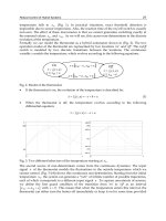
Under these conditions, the principles of control used in the past (cartographic approach,
buckles open…) are not enough sufficient. Indeed, the output variables (quantity injected,
advances in lighting or in injection) were primarily given starting from two variables of
entry (speed and load). Today, the use of new technologies in the conception of engines, in
order to reduce the pollutant emissions, as for example EGR (exhaust Gas Recirculation)
(Pierpont et al. 1995), multiply the number of parameters to control, as we can see it in Fig.1.
This figure shows the exponential evolution of number of setting parameters due to the
hardware complexity increase. This makes the cartographic approach impracticable.
Moreover, this kind of approach does not take into account the dynamic of system.
The main drawback of this evolution is the increase of the difficulty to understand the
engine behavior. To deals with all the parameters, we use a Kriging model which we define
in the next section.
Fig. 1. Parameters to tune a diesel engine function of technologies
3. Ordinary Kriging Techniques
Kriging methods are used frequently for spatial interpolation of soil properties (Krige, 1951;
Matheron, 1963). Kriging is a linear least squares estimation algorithm. It is a tool for
interpolation. The aim is to estimate the value of an unknown real function ܼ at pointݔ
כ
,
given the values of function ܼ
at some other points ݔ
אܴ
ௗ
for each݅ൌͳǡǥǡ݊
.
TwostageapproachesformodelingpollutantemissionofdieselenginebasedonKrigingmodel 31
significant estimate of its parameters, and we are very limited by the small experiments
number which the industrialist is able to realize. The techniques of the design of
experiments (Cochran & Cox, 1957) were conceived to deal with this kind of problems. On
the other hand, recent works (Sacks et al. 1989; Bates et al. 1996; Koehler & Owen, 1996)
suggest that the polynomial models are not adapted to the numerical experiments. For
example, a surface of response of order two is not enough flexible to model a surface
admitting several extrema.
The aim of this paper is to present the result that we have obtained in the field of pollutants
emissions prediction. These results were obtained without the increase of the number of the
experiments that the industrialist can do. We call upon a sophisticated statistical model
resulting from the field of geostatistic named Kriging.
We use this method, through two approaches, in order to improve the prediction of NOx
(nitrogen oxide) emissions, and fuel consumption.
In the first stage, we estimate the response directly from the controllable factors like main
injection timing, pressure in common rail. This can be assimilated to a black box modelling.
In the second stage, we propose an innovative approach that allows us to predict the
response from a functional data. More precisely, we estimate the engine performance from
signals like pressure and cylinder temperature. These signals are obtained from a model of
combustion. The main advantage of the second approach is that it allows us to include a
physical knowledge of combustion. This lack of knowledge is often criticized in the case of
black boxes models.
The Kriging method is very well adapted for the second approach which predicts engine
responses from the state variables (signals) obtained from a physical model of combustion.
This means that this method can be recommended in cases where we have a lot of decision
variables, with a small number of experiences. This is due to the fact that the method is
based on the study of the similarity of the response of interest in different sites, in relation to
the distance separating them. We recall that, Software such as R and Matlab contain a
toolbox to use this method. But unfortunately, the latter are restricted to less than 3
dimensions. Adapting the method to higher dimensions has been considered.
To implement this second approach, a model reduction is needed. This reduction will be
made in two steps:
1) Reducing the number of state variables from 10 to 2 by the study of correlations.
2) Reducing the number of points in each signal using the theory of Fourier.
Once the reduction is made, the Kriging can be applied to the model obtained.
This paper is organized as follows: In the second section, we describe the engine behaviour
and recall the importance of controlling pollutant emissions. In the third section, the
ordinary Kriging techniques are recalled. In the fourth section, two different approaches for
modelling our problem are proposed. An efficient reduction model strategy is considered in
order to apply the Kriging method. Finally, the Kriging method is applied to the reduced
model. In the last section, numerical results are given followed by a short discussion.
2. Engine calibration
The engine calibration is a process which aims at defining the values of the engine control
parameters. During the ten last years, the set of themes “engine calibration” took an
important place in the process of the development of the internal combustion engines.
Indeed, under the impulse of the standards more and more severe, the car manufacturers
are brought to integrate more and more elaborated technologies in the power unit.
Under these conditions, the principles of control used in the past (cartographic approach,
buckles open…) are not enough sufficient. Indeed, the output variables (quantity injected,
advances in lighting or in injection) were primarily given starting from two variables of
entry (speed and load). Today, the use of new technologies in the conception of engines, in
order to reduce the pollutant emissions, as for example EGR (exhaust Gas Recirculation)
(Pierpont et al. 1995), multiply the number of parameters to control, as we can see it in Fig.1.
This figure shows the exponential evolution of number of setting parameters due to the
hardware complexity increase. This makes the cartographic approach impracticable.
Moreover, this kind of approach does not take into account the dynamic of system.
The main drawback of this evolution is the increase of the difficulty to understand the
engine behavior. To deals with all the parameters, we use a Kriging model which we define
in the next section.
Fig. 1. Parameters to tune a diesel engine function of technologies
3. Ordinary Kriging Techniques
Kriging methods are used frequently for spatial interpolation of soil properties (Krige, 1951;
Matheron, 1963). Kriging is a linear least squares estimation algorithm. It is a tool for
interpolation. The aim is to estimate the value of an unknown real function ܼ at pointݔ
כ
,
given the values of function ܼ
at some other points ݔ
אܴ
ௗ
for each݅ൌͳǡǥǡ݊
.
AUTOMATION&CONTROL-TheoryandPractice32
3.1 Ordinary Kriging
The ordinary Kriging estimator
is defined by:
(1)
Where n is the number of surrounding observations
and
is the weight of
. The
weights should sum to unity in order to make the estimator unbiased:
(2)
The weights are also determined such that the following Kriging variance is minimal under
the constraint given by the equation 2:
This leads to a classical optimization problem with equality constraint. The Lagrange
multiplier theory is used in order to work out this problem. This gives a linear system which
must solved (Davis, 1986).
3.2 Variogram
The variogram is a function representing the spatial dependency. It is obtained from the
stationarity definition. In fact, this stationarity hypothesis is an indispensable condition for
the use of the Kriging method.
In the case of ordinary Kriging the expression of the variogram is obtained from the
following definition of intrinsic stationarity:
1)
2)
More precisely, the expression of the theoretical variogram, is deduced from the second
condition of intrinsic stationarity. This condition means that the variation of a data set is
only dependent on distance r between two locations, where the variables values are
and
with
.
Note that the variogram,
, is a function of the separation between points and not a
function of the specific location
. This mathematical definition is a useful
abstraction, but not easy to apply to observed values.
Consider a set of n observed data:
where
is the location of
observation and
is the associated observed value. There are
unique pairs of
observations. For each of these pairs we can calculate the associated separation distance:
To infer the variogram from observed data, we will then use the common formula for the
experimental variogram (Cressie, 1993).
(3)
Where:
is the pair number of
and
;
is the experimental variogram.
3.3 Variogram Modeling
The experimental variogram presented in equation 3, estimates the theoretical variogram,
for only a finite number of distances. Moreover, it does not necessarily form a valid
variogram. This means, that maybe, it does not concern a negative conditionally function.
Indeed, this condition is necessary to ensure the positivity of the variance of a sum of
random variables (Christakos, 1984).
The experimental variogram is then modeled by a function of negative conditional type and
is defined for all distances. This modeling makes the Kriging possible. A variogram model
should be fitted to such variogram.
A model must be selected among the various forms of the variogram models which exist in
the literature and adjusted of experimental variogram (Arnaud & Emery, 2000 ). This means
that the parameters of the model must be estimated. This adjustment can be done
graphically, but it is usually done with an estimation method such as the weighted least
squares or maximum likelihood method.
Once the variographic model is chosen, and its parameters are estimated, we compute the
weights
which appear
in (1) by solving the following system:
, with
(4)
And
Where is the Lagrange multiplier.
is the variogram model used for adjusting the experimental variogram.
is the distance between the locations
and
.
The variance of the estimate
i.e. the square of the standard error at each point is obtained
by the relationship:
If we assume that the estimation errors are normally distributed around the true value, then
the probability that the true value will be in
is 68 %, while the probability that the
true value will be in
is 95 %, (Davis, 1986).
3.4 Kriging Emulator Validation
The true test of the quality of the fitted emulator model is its ability to predict the response
at untried factor values. In order to maximally exploit the data to aid model fitting, the
emulators are validated using leave-one-out cross validation. This process involves taking
the fitted model and re-fitting it to a subset of non used experimental data.
More precisely, for an experiment with d design factors
, the set of n
experimental design points
and responses
, contain the
information used to build the Kriging model. A cross validation involves predicting at each
design point in turn when that point is left out of the predictor equations. Let
be the
TwostageapproachesformodelingpollutantemissionofdieselenginebasedonKrigingmodel 33
3.1 Ordinary Kriging
The ordinary Kriging estimator
is defined by:
(1)
Where n is the number of surrounding observations
and
is the weight of
. The
weights should sum to unity in order to make the estimator unbiased:
(2)
The weights are also determined such that the following Kriging variance is minimal under
the constraint given by the equation 2:
This leads to a classical optimization problem with equality constraint. The Lagrange
multiplier theory is used in order to work out this problem. This gives a linear system which
must solved (Davis, 1986).
3.2 Variogram
The variogram is a function representing the spatial dependency. It is obtained from the
stationarity definition. In fact, this stationarity hypothesis is an indispensable condition for
the use of the Kriging method.
In the case of ordinary Kriging the expression of the variogram is obtained from the
following definition of intrinsic stationarity:
1)
2)
More precisely, the expression of the theoretical variogram, is deduced from the second
condition of intrinsic stationarity. This condition means that the variation of a data set is
only dependent on distance r between two locations, where the variables values are
and
with
.
Note that the variogram,
, is a function of the separation between points and not a
function of the specific location
. This mathematical definition is a useful
abstraction, but not easy to apply to observed values.
Consider a set of n observed data:
where
is the location of
observation and
is the associated observed value. There are
unique pairs of
observations. For each of these pairs we can calculate the associated separation distance:
To infer the variogram from observed data, we will then use the common formula for the
experimental variogram (Cressie, 1993).
(3)
Where:
is the pair number of
and
;
is the experimental variogram.
3.3 Variogram Modeling
The experimental variogram presented in equation 3, estimates the theoretical variogram,
for only a finite number of distances. Moreover, it does not necessarily form a valid
variogram. This means, that maybe, it does not concern a negative conditionally function.
Indeed, this condition is necessary to ensure the positivity of the variance of a sum of
random variables (Christakos, 1984).
The experimental variogram is then modeled by a function of negative conditional type and
is defined for all distances. This modeling makes the Kriging possible. A variogram model
should be fitted to such variogram.
A model must be selected among the various forms of the variogram models which exist in
the literature and adjusted of experimental variogram (Arnaud & Emery, 2000 ). This means
that the parameters of the model must be estimated. This adjustment can be done
graphically, but it is usually done with an estimation method such as the weighted least
squares or maximum likelihood method.
Once the variographic model is chosen, and its parameters are estimated, we compute the
weights
which appear
in (1) by solving the following system:
, with
(4)
And
Where is the Lagrange multiplier.
is the variogram model used for adjusting the experimental variogram.
is the distance between the locations
and
.
The variance of the estimate
i.e. the square of the standard error at each point is obtained
by the relationship:
If we assume that the estimation errors are normally distributed around the true value, then
the probability that the true value will be in
is 68 %, while the probability that the
true value will be in
is 95 %, (Davis, 1986).
3.4 Kriging Emulator Validation
The true test of the quality of the fitted emulator model is its ability to predict the response
at untried factor values. In order to maximally exploit the data to aid model fitting, the
emulators are validated using leave-one-out cross validation. This process involves taking
the fitted model and re-fitting it to a subset of non used experimental data.
More precisely, for an experiment with d design factors
, the set of n
experimental design points
and responses
, contain the
information used to build the Kriging model. A cross validation involves predicting at each
design point in turn when that point is left out of the predictor equations. Let
be the
AUTOMATION&CONTROL-TheoryandPractice34
estimate of the
based on all the design points except
. The prediction error (the
estimated root mean square error, RMSE) is then calculated as:
(5)
An index of the accuracy of the emulator is made by expressing as a percentage of the range
of the response,
(6)
4. Two approaches to model engine responses
In this section we present two stage approaches based on Kriging method for the prediction
of NOx (nitrogen oxide) emissions, and fuel consumption.
In the first stage, we estimate the response directly from the controllable factor like main
injection timing, pressure in common rail (black box).
In the second stage, we propose an innovative approach that allows us to predict the engine
response from signals, like pressure and cylinder temperature (states variables of
combustion chamber).
4.1 First approach
We recall that the first approach consists to build a Kriging model from the controllable
parameters. Thus, the Kriging was trained on about 300 input/ output sets of points
generated by using D-optimal design method. The training examples cover engine speeds
from 1000 rpm to 5000 rpm in 250 rpm intervals, and load vary from 1 to 23 bar. The data
was generated to cover the cycle point of the engine map in order to construct a global
Kriging emulator. For this reason, our model takes into account the engine speed among the
following control parameters:
Prail : rail pressure, - Main: Main injection quantity,
Mpil1: pilot1 injection quantity, - Pmain: Main injection timing,
Mpil2: pilot2 injection quantity, - Ppil2: pilot2 injection timing,
Ppil1: pilot1 injection timing, -VNT: turbine vane position,
VEGR: EGR valve position, - Volet: position component of admission,
4.2 Second approach
4.2.1 Modelling
In the second approach, we propose an innovative approach that allows us to predict the
response from signals like pressure and cylinder temperature (states variables of
combustion chamber).
More precisely, we decompose the problem of estimation of the engine responses, into two
steps sub problems (Fig.2):
Fig. 2. Coupling of the pollutants and consumption models with the combustion model.
1) The first step consists in simulating the various thermodynamic quantities from a
physical model. In this work, we use the model developed by
(Castric et al., 2007), which
takes into account the input parameters. It leads to have a good representation of the
experimental results. This model allows us to generate the following thermodynamic
quantities:
The cylinder low pressure (the alone quantity that we can measure)
The temperature in the cylinder,
The temperature of the fresh gas in the cylinder
The temperature of the mixed gas in the cylinder,
The temperature of the burned gas in the cylinder,
The mass of the fresh gas in the cylinder,
The mass of the entrained gas in the cylinder,
The mass of the burned gas in the cylinder,
The turbulence in the motor,
The fuel vapor mass.
We precise, that each signal is represented by a vector of 1334 components.
2) The second step consists in building a statistical Kriging model, from the 11
thermodynamics quantities generated by the model of combustion.
It is true that the advantage of this procedure is that, it allows us to include a physical
knowledge of combustion. But this approach requires a great time of computing. Indeed to
build Kriging from 11 signals, can pose a serious problem in memory capacity and the
computing time can be considerable. Thus, to be able to implement this procedure, a
reduction of the model is essential.
ሻࢎ࢙࢟ࢉࢇࢊࢋ
ᇣ
ᇧ
ᇧ
ᇧ
ᇧ
ᇧ
ᇤ
ᇧ
ᇧ
ᇧ
ᇧ
ᇧ
ᇥ
ሻ࢙࢚ࢇ࢚࢙࢚ࢉࢇࡷ࢘ࢍࢍࢊࢋ
ᇣ
ᇧ
ᇧ
ᇧ
ᇧ
ᇧ
ᇧ
ᇧ
ᇧ
ᇧ
ᇧ
ᇤ
ᇧ
ᇧ
ᇧ
ᇧ
ᇧ
ᇧ
ᇧ
ᇧ
ᇧ
ᇧ
ᇥ
TwostageapproachesformodelingpollutantemissionofdieselenginebasedonKrigingmodel 35
estimate of the
based on all the design points except
. The prediction error (the
estimated root mean square error, RMSE) is then calculated as:
(5)
An index of the accuracy of the emulator is made by expressing as a percentage of the range
of the response,
(6)
4. Two approaches to model engine responses
In this section we present two stage approaches based on Kriging method for the prediction
of NOx (nitrogen oxide) emissions, and fuel consumption.
In the first stage, we estimate the response directly from the controllable factor like main
injection timing, pressure in common rail (black box).
In the second stage, we propose an innovative approach that allows us to predict the engine
response from signals, like pressure and cylinder temperature (states variables of
combustion chamber).
4.1 First approach
We recall that the first approach consists to build a Kriging model from the controllable
parameters. Thus, the Kriging was trained on about 300 input/ output sets of points
generated by using D-optimal design method. The training examples cover engine speeds
from 1000 rpm to 5000 rpm in 250 rpm intervals, and load vary from 1 to 23 bar. The data
was generated to cover the cycle point of the engine map in order to construct a global
Kriging emulator. For this reason, our model takes into account the engine speed among the
following control parameters:
Prail : rail pressure, - Main: Main injection quantity,
Mpil1: pilot1 injection quantity, - Pmain: Main injection timing,
Mpil2: pilot2 injection quantity, - Ppil2: pilot2 injection timing,
Ppil1: pilot1 injection timing, -VNT: turbine vane position,
VEGR: EGR valve position, - Volet: position component of admission,
4.2 Second approach
4.2.1 Modelling
In the second approach, we propose an innovative approach that allows us to predict the
response from signals like pressure and cylinder temperature (states variables of
combustion chamber).
More precisely, we decompose the problem of estimation of the engine responses, into two
steps sub problems (Fig.2):
Fig. 2. Coupling of the pollutants and consumption models with the combustion model.
1) The first step consists in simulating the various thermodynamic quantities from a
physical model. In this work, we use the model developed by
(Castric et al., 2007), which
takes into account the input parameters. It leads to have a good representation of the
experimental results. This model allows us to generate the following thermodynamic
quantities:
The cylinder low pressure (the alone quantity that we can measure)
The temperature in the cylinder,
The temperature of the fresh gas in the cylinder
The temperature of the mixed gas in the cylinder,
The temperature of the burned gas in the cylinder,
The mass of the fresh gas in the cylinder,
The mass of the entrained gas in the cylinder,
The mass of the burned gas in the cylinder,
The turbulence in the motor,
The fuel vapor mass.
We precise, that each signal is represented by a vector of 1334 components.
2) The second step consists in building a statistical Kriging model, from the 11
thermodynamics quantities generated by the model of combustion.
It is true that the advantage of this procedure is that, it allows us to include a physical
knowledge of combustion. But this approach requires a great time of computing. Indeed to
build Kriging from 11 signals, can pose a serious problem in memory capacity and the
computing time can be considerable. Thus, to be able to implement this procedure, a
reduction of the model is essential.
ሻࢎ࢙࢟ࢉࢇࢊࢋ
ᇣ
ᇧ
ᇧ
ᇧ
ᇧ
ᇧ
ᇤ
ᇧ
ᇧ
ᇧ
ᇧ
ᇧ
ᇥ
ሻ࢙࢚ࢇ࢚࢙࢚ࢉࢇࡷ࢘ࢍࢍࢊࢋ
ᇣ
ᇧ
ᇧ
ᇧ
ᇧ
ᇧ
ᇧ
ᇧ
ᇧ
ᇧ
ᇧ
ᇤ
ᇧ
ᇧ
ᇧ
ᇧ
ᇧ
ᇧ
ᇧ
ᇧ
ᇧ
ᇧ
ᇥ
AUTOMATION&CONTROL-TheoryandPractice36
4.2.2 Model reduction
The data of the first model can be directly used for the Kriging. It is not the case for the
second one. In the last case the data have to be reduced.
The reduction process begins by studying the different correlations between the state
variables and their corresponding p-value. The chosen criterion consists in testing the p-
value: if it is less than to 0.05, the correlation is significant. This analysis allows us to retain
only two state variables: the cylinder pressure and the mixed gas temperature in the
cylinder, Te.
In the second step, the number of components of the two remaining signals is reduced. This
is accomplished by using the discrete Fourier transform. The function fft of Matlab returns
the discrete Fourier transform (DFT) of a vector, computed with a fast Fourier transform
(FFT) algorithm. After calculating the coefficients, a minimum number of them are retained.
This allows us to reproduce the initial signal, with a relative error approximately less than
0.02.
The reduction of the number of points of each signal is tantamount to minimize the number
of Fourier coefficients representing that signal. The two retained signals representing
respectively the cylinder pressure and the temperature of the mixed gas in the cylinder,
have been reduced to a 40 Fourier coefficients. Each signal has been reconstructed from the
40 kept coefficients, with an acceptable relative error. The following table.1 presents the
relative error committed, for the reconstruction of the two signals from the 40 coefficients
selected:
Relative error =
S: is the experimental signal
is the reconstruction of the signal S using the fast Fourier transformation.
is the Euclidian norm.
Type of signal relative
error
the cylinder low pressure
0.01
the temperature of the mixed gas in the cylinder
0.02
Table 1. Relative error committed for the reconstruction of two signals.
Figure 3 shows the experimental signals, resulting from the combustion and their
reconstruction by using the fft Matlab function.
Fig. 3 Rebuilding of the measured signals (red curve) by using the discrete Fourier
transform (blue curve)
Such reduction makes the Kriging possible. The considered entries of the model are:
Where:
i is the index that corresponds to the ith operating point of engine. An operation point of the
engine is defined by engine speed and engine torque
is the kept Fourier coefficient for the signal, which corresponds to the ith operating
point of engine.
5. Application to the estimation of engine responses
In the previous section, we have presented and explained the two approaches used in this
work, in order to model a behavior of diesel engine. Then, this section will be devoted to
present the results respectively obtained by each approach, for the estimation of each
response.
5.1 Numerical results using the first approach
We recall that the construction and the modeling of the experimental variogram is the most
important step in the Kriging method. Thus, in this part, we will start by giving the chosen
model.
Variogram fitting:
Variography modeling is a critical step and most difficult in the construction of a Kriging
model. For this reason, several models were adjusted and then compared. It was difficult to
select the better model graphically. The cross validation facilitates the work. It allows us to
select the one, which minimizes the root mean square error.
Pressure
Temperature
TwostageapproachesformodelingpollutantemissionofdieselenginebasedonKrigingmodel 37
4.2.2 Model reduction
The data of the first model can be directly used for the Kriging. It is not the case for the
second one. In the last case the data have to be reduced.
The reduction process begins by studying the different correlations between the state
variables and their corresponding p-value. The chosen criterion consists in testing the p-
value: if it is less than to 0.05, the correlation is significant. This analysis allows us to retain
only two state variables: the cylinder pressure and the mixed gas temperature in the
cylinder, Te.
In the second step, the number of components of the two remaining signals is reduced. This
is accomplished by using the discrete Fourier transform. The function fft of Matlab returns
the discrete Fourier transform (DFT) of a vector, computed with a fast Fourier transform
(FFT) algorithm. After calculating the coefficients, a minimum number of them are retained.
This allows us to reproduce the initial signal, with a relative error approximately less than
0.02.
The reduction of the number of points of each signal is tantamount to minimize the number
of Fourier coefficients representing that signal. The two retained signals representing
respectively the cylinder pressure and the temperature of the mixed gas in the cylinder,
have been reduced to a 40 Fourier coefficients. Each signal has been reconstructed from the
40 kept coefficients, with an acceptable relative error. The following table.1 presents the
relative error committed, for the reconstruction of the two signals from the 40 coefficients
selected:
Relative error =
S: is the experimental signal
is the reconstruction of the signal S using the fast Fourier transformation.
is the Euclidian norm.
Type of signal relative
error
the cylinder low pressure
0.01
the temperature of the mixed gas in the cylinder
0.02
Table 1. Relative error committed for the reconstruction of two signals.
Figure 3 shows the experimental signals, resulting from the combustion and their
reconstruction by using the fft Matlab function.
Fig. 3 Rebuilding of the measured signals (red curve) by using the discrete Fourier
transform (blue curve)
Such reduction makes the Kriging possible. The considered entries of the model are:
Where:
i is the index that corresponds to the ith operating point of engine. An operation point of the
engine is defined by engine speed and engine torque
is the kept Fourier coefficient for the signal, which corresponds to the ith operating
point of engine.
5. Application to the estimation of engine responses
In the previous section, we have presented and explained the two approaches used in this
work, in order to model a behavior of diesel engine. Then, this section will be devoted to
present the results respectively obtained by each approach, for the estimation of each
response.
5.1 Numerical results using the first approach
We recall that the construction and the modeling of the experimental variogram is the most
important step in the Kriging method. Thus, in this part, we will start by giving the chosen
model.
Variogram fitting:
Variography modeling is a critical step and most difficult in the construction of a Kriging
model. For this reason, several models were adjusted and then compared. It was difficult to
select the better model graphically. The cross validation facilitates the work. It allows us to
select the one, which minimizes the root mean square error.
Pressure
Temperature
AUTOMATION&CONTROL-TheoryandPractice38
For the NOx, the retained model is a Gaussian model which is expressed by the equation:
(7)
The value of the model parameters was founded using the least square method. So, we
obtain:
=10.929, c=1.829, a=309.559.
For the Consumption, the model used is an exponential model, given by the equation:
(8)
This leads to:
=7.106, c=2.415, a=477.444.
Where:
r is the distance
is the Nugget effect
is the sill correspond to the variance of
and 3a are the range (the distance at which the variogram reaches the sill) for the
Gaussian and exponential model respectively (Baillargeon et al., 2004).
Figures 4 shows the experimental variogram (red points), and Gaussian model (blue curve)
corresponding to NOx response.
Figures 5 shows the experimental variogram (red points), and exponential model (blue
curve) corresponding to consumption response.
The variogram is the tool which quantifies the spatial correlation of the response in of
interest. It measures the variability of NOx and consumption as a function of distance. We
notice that, when the distance reaches the range
(Fig.4) and (Fig.5),
the variation becomes stationary. This explains why we can have a similar behavior of
consumption and NOx on two different operating points, thus with a pattern of different
control parameters
Fig. 4. and Fig. 5. Experimental and model variogram
Fig. 5. Experimental and exponential
model variogram in the case of
consumption
Fig. 4. Experimental and Gaussian
model variogram in the case of NOx
Figures 6 and 7 show the Cross-validation plots for the Kriging model, corresponding to the
Gaussian and exponential variogram respectively. The plots contain the measured, the
Kriging estimated value and a 10% errors bands
.
The accuracy of predictions was similar for both validation data. Accuracy was good for
both of the responses and still within 10% for the majority of operating conditions.
By against, graph 7 presents some observations which are poorly estimated. This is because
they are far from the cloud of points used for the adjustment. This bad estimate is also due
to the experimental design used. The classical and optimal designs, in particular the D-
optimal, are not suitable for Kriging, which is based on measuring similarity between sites.
Indeed, the D-optimal design allows to test just a small number of levels for each variable
and tend to generate points on the edges of the experimental field (Koehler & Owen, 1996).
This distribution of points, which is optimal to fit a polynomial model, cannot pick up any
irregularities inside the experimental field and lead to some poorly estimated points. To
address this problem, we recommend to use an appropriate designs for Kriging. Class
’space filling designs’, such as Latin hypercubes, provide a good spatial distribution of
points and is well adapted for modeling by Kriging (Stein, 1987), (McKay et al., 2000).
Fig. 6. Measured and Kriging predicted NOx [ppm] with ± 10% error bands
TwostageapproachesformodelingpollutantemissionofdieselenginebasedonKrigingmodel 39
For the NOx, the retained model is a Gaussian model which is expressed by the equation:
(7)
The value of the model parameters was founded using the least square method. So, we
obtain:
=10.929, c=1.829, a=309.559.
For the Consumption, the model used is an exponential model, given by the equation:
(8)
This leads to:
=7.106, c=2.415, a=477.444.
Where:
r is the distance
is the Nugget effect
is the sill correspond to the variance of
and 3a are the range (the distance at which the variogram reaches the sill) for the
Gaussian and exponential model respectively (Baillargeon et al., 2004).
Figures 4 shows the experimental variogram (red points), and Gaussian model (blue curve)
corresponding to NOx response.
Figures 5 shows the experimental variogram (red points), and exponential model (blue
curve) corresponding to consumption response.
The variogram is the tool which quantifies the spatial correlation of the response in of
interest. It measures the variability of NOx and consumption as a function of distance. We
notice that, when the distance reaches the range
(Fig.4) and (Fig.5),
the variation becomes stationary. This explains why we can have a similar behavior of
consumption and NOx on two different operating points, thus with a pattern of different
control parameters
Fig. 4. and Fig. 5. Experimental and model variogram
Fig. 5. Experimental and exponential
model variogram in the case of
consum
p
tion
Fig. 4. Experimental and Gaussian
model variogram in the case of NOx
Figures 6 and 7 show the Cross-validation plots for the Kriging model, corresponding to the
Gaussian and exponential variogram respectively. The plots contain the measured, the
Kriging estimated value and a 10% errors bands
.
The accuracy of predictions was similar for both validation data. Accuracy was good for
both of the responses and still within 10% for the majority of operating conditions.
By against, graph 7 presents some observations which are poorly estimated. This is because
they are far from the cloud of points used for the adjustment. This bad estimate is also due
to the experimental design used. The classical and optimal designs, in particular the D-
optimal, are not suitable for Kriging, which is based on measuring similarity between sites.
Indeed, the D-optimal design allows to test just a small number of levels for each variable
and tend to generate points on the edges of the experimental field (Koehler & Owen, 1996).
This distribution of points, which is optimal to fit a polynomial model, cannot pick up any
irregularities inside the experimental field and lead to some poorly estimated points. To
address this problem, we recommend to use an appropriate designs for Kriging. Class
’space filling designs’, such as Latin hypercubes, provide a good spatial distribution of
points and is well adapted for modeling by Kriging (Stein, 1987), (McKay et al., 2000).
Fig. 6. Measured and Kriging predicted NOx [ppm] with ± 10% error bands
AUTOMATION&CONTROL-TheoryandPractice40
Fig. 7. Measured and Kriging predicted consumption [g/kWh] with ± 10% error bands
The emulator model is fitted to each response in turn and the RMSE, percentage RMSE are
recorded. These results are presented in Table2. The percentage RMSE results show that the
model has a %RMSE less than 7% of the range of the response data. This indicates roughly,
that if the emulator is used to predict the response at a new input setting, the error of
prediction can be expected to be less than 7%, when compared with the true value.
NOx Consumption
RMSE 61.4 40.63
%RMSE 3.84 6.19
Table 2. Kriging RMSE end %RMSE for each response: first approach case
5.2 Numerical results using the second approach
This subsection is devoted to the presentation of the numerical results obtained in the case
of the second modeling. More precisely, we give the mathematical model used to adjust the
experimental variogram.
Variogram fitting:
The experimental variogram and the model which adjusts it for each response, were
obtained by the same way that we have used in the first approach case.
For the NOx, the model used is a power model given by equation:
ߛ
ሺ
ݎ
ሻ
ൌܿ
ܿݎ
ܽݏݎͲܽ݊݀Ͳܽ൏ʹ (9)
The value of the model parameters was founded using the least square method.
So, c0=997.28, c=0.00018, a=1.52.
In this case the variogram does not show a sill. This means that the variance does not exist.
For the consumption, the model used is an exponential model given by equation:
(10)
So
=5193, c=0.0327, a=5.9536
Where:
r is the distance.
is the Nugget effect.
is the sill correspond to the variance of
.
3a is the range (the distance at which the variogram reaches the sill) for the exponential
model (Baillargeon et al., 2004).
Figures 8 shows the experimental variogram (red points), and power model (blue curve)
corresponding to NOx response.
Figures 9 shows the experimental variogram (red points), and exponential model (blue
curve) corresponding to consumption response.
We notice that when the distance reaches the range (Fig. 9), the variation
becomes stationary. In other term, this means that there is no correlation beyond the
distance 3a. This explains that we have a similar behavior of consumption on two different
operating points, thus with a pattern of different control parameters.
Let us notice that the model used here for the variogram of NOx, is of power type, contrary
to what we had made in the first approach, where the Gaussian model was retained.
This explains that different engine configurations, lead to different behavior of the NOx.
More details will be given in the section 6.
Fig. 8. and Fig. 9. Experimental and model variogram
Figures 10 and 11 show the cross-validation plots for the Kriging model, corresponding to
the power and exponential variogram respectively. The plots contain the measured, the
Kriging estimated value and a 10% errors bands.
As we can see it, the accuracy of the predictions is similar for both response and still within
10% for the majority of operating conditions.
Fig. 9. Experimental and exponential
model variogram in the case of
consumption
Fig. 8. Experimental and power
model variogram in the case of NOx