industrial control

Contents

Hong Kong IGDS 2000
Industrial Control

Table of Contents

● Chapter 0 - Introductions
● Chapter 1 - Sensors
● Chapter 2 - Actuators
● Chapter 3 - Industrial Electronic
● Chapter 4 - Motor Drives
● Chapter 5 - Control Components
● Chapter 6 - Sequential Logic
● Chapter 7 - Programmable Logic Controllers
● Chapter 8 - Computer Control Systems
● Chapter 9 - Computer Interface
● Chapter 10 - Real Time Control Platform
● Chapter 11 - Sstems Modelling
● Chapter 12 - Servo Control

Time Table

End
Chapter 0. Introduction
Chapter 0. INTRODUCTION

0.1 AUTOMATE, EMIGRATE, LEGISLATE, OR
EVAPORATE
"Automate, emigrate, legislate or evaporate." This was a choice many manufacturers.
Some manufacturers tried to lower prices by reducing manufacturing costs. They either automated or emigrated.

Many countries legislated trade barriers to keep high quality, low cost products out. Manufacturers who did nothing
disappeared, often despite their own government's protective trade barriers.
Many consumers still choose imports over domestic products, but some North American manufacturers are now
trying more thoughtful measures to meet the challenge.
Automation is a technique that can be used to reduce costs and/or to improve quality. Automation can increase
manufacturing speed, while reducing cost. Automation can lead to products having consistent quality, perhaps even
consistently good quality. Some manufacturers who automated survived. Others didn't. The ones who survived
were those who used automation to improve quality. It often happened that improving quality led to reduced costs.

0.2 THE ENVIRONMENT FOR AUTOMATION
Automation, the subject of this textbook, is not a magic solution to financial problems. It is, however, a valuable
tool that can be used to improve product quality. Improving product quality, in turn, results in lower costs.
Producing inexpensive, high quality products is a good policy for any company.
But where do you start?
Simply considering an automation program can force an organization to face problems it might not otherwise face:
● What automation and control technology is available?
● Are employees ready and willing to use new technology?
● What technology should we use?
● Should the current manufacturing process be improved before automation?
● Should the product be improved before spending millions of dollars acquiring equipment to build it?
Automating before answering the above questions would be foolish. The following chapters describe the available
technology so that the reader will be prepared to select appropriate automation technology. The answers to the last
two questions above are usually "yes," and this book introduces techniques to improve processes and products, but
each individual organization must find its own improvements.
Chapter 0. Introduction

0.2.1 Automated Manufacturing, an Overview
Automating of individual manufacturing cells should be the second step in a three step evolution to a different
manufacturing environment. These steps are:
1. Simplification of the manufacturing process. If this step is properly managed, the other two steps

might not even be necessary. The "Just In Time" (JIT) manufacturing concept includes procedures
that lead to a simplified manufacturing process.
2. Automation of individual processes. This step, the primary subject of this text, leads to the
existence of "islands of automation" on the plant floor. The learning that an organization does at this
step is valuable. An organization embarking on an automation program should be prepared to accept
some mistakes in the early stage of this phase. The cost of those mistakes is the cost of training
employees.
3. Integration of the islands of automation and other computerized processes into a total
manufacturing and business system. While this text does not discuss the details of integrated
manufacturing, it is discussed in general in this chapter and again. Technical specialists should be
aware of the potential future need to integrate, even while they embark on that first "simplification"
step.
The large, completely automated and integrated environment shown in figure 0.1 is a Computer Integrated
Manufacturing (CIM) operation. The CIM operation includes:
● Computers, including:
i one or more "host" computers
ii several cell controller computers
iii a variety of personal computers
iv Programmable Controllers (PLC)
v computer controllers built into other equipment
● Manufacturing Equipment, including:
i robots
ii numerical control machining equipment (NC, CNC, or DNC)
iii conntrolled continuous process equipment (e.g., for turning wood pulp into paper)
iv assorted individual actuators under computer control (e.g., motorized conveyor systems)
v assorted individual computer-monitored sensors (e.g., conveyor speed sensors)
vi
pre-existing "hard" automation equipment, not properly computer-controllable, but
monitored by retro-fitted sensors
● Computer Peripherals, such as:

i printers, FAX machines, terminals, paper-tape printers, etc.
Chapter 0. Introduction
● Local Area Networks (LANs) interconnecting computers, manufacturing equipment, and shared
peripherals. "Gateways" may interconnect incompatible LANs and incompatible computers.

● Databases (DB), stored in the memories of several computers, and accessed through a Database
Management System (DBMS)

● Software Packages essential to the running of the computer system. Essential software would include: the
operating system(s) (e.g., UNIX, WINDOWS NT, OS/2 or SNA) at each computer; communications
software (e.g., the programs which allow the LANs to move data from computer to computer and which
allow some controllers to control other controllers); and the database management system (DBMS)
programs

● assorted "processes" which use the computers. These computer- users might include:
i
humans, at computer terminals, typing commands or receiving information
from the computers
ii Computer Aided Design (CAD) programs
iii Computer Aided Engineering (CAE) programs
iv
Computer Aided Manufacturing (CAM) programs, including those that do
production scheduling (MRP), process planning (CAPP), and monitoring of
shop floor feedback and control of manufacturing processes (SEC)
v
miscellaneous other programs for uses such as word processing or financial
accounting

As of this writing, very few completely computer integrated manufacturing systems are in use. There are lots of
partially integrated manufacturing systems. Before building large computer integrated systems, we must first

understand the components and what each component contributes to the control of a simple process.

Chapter 0. Introduction

Fig. 0.1 A computer integrated manufacturing environment

0.3 CONTROL OF AUTOMATION/PROCESS CONTROL
Automated processes can be controlled by humans operators, by computers, or by a combination of the two. If a
human operator is available to monitor and control a manufacturing process, open loop control may be acceptable.
If a manufacturing process is automated, then it requires closed loop control.
Chapter 0. Introduction
Figure 0.2 shows examples of open loop control and closed loop control. One major difference is the presence of
the sensor in the closed loop control system. The motor speed controller uses the feedback it receives from this
sensor to verify that the speed is correct, and drives the actuator harder or softer until the correct speed is achieved.
In the open loop control system, the operator uses his/her built-in sensors (eyes, ears, etc.) and adjusts the actuator
(via dials, switches, etc.) until the output is correct. Since the operator provides the sensors and the intelligent
control functions, these elements do not need to be built into an open loop manufacturing system.
Human operators are more inconsistent than properly programmed computers. Anybody who has ever shared the
road with other drivers is familiar with the disadvantages of human control. Computerized controls, however, can
also make mistakes, when programmed to do so. Programming a computer to control a complex process is very
difficult (which is why human automobile operators have not yet been replaced by computers).
The recent development of affordable digital computers has made automation control possible. Process control has
been around a little longer. The difference in the meanings of these two terms is rapidly disappearing.
Process control usually implies that the product is produced in a continuous stream. Often, it is a liquid that is being
processed. Early process control systems consisted of specially-designed analog control circuitry that measured a
system's output (e.g., the temperature of liquid leaving a tank), and changed that output (e.g., changing the amount
of cool liquid mixed in) to force the output to stay at a preset value.


Fig. 0.2 Open loop and closed loop speed control

Automation control usually implies a sequence of mechanical steps. A camshaft is an automation controller
because it mechanically sequences the steps in the operation of an internal combustion engine. Manufacturing
processes are often sequenced by special digital computers, known as programmable logic controllers (PLCs),
which can detect and can switch electrical signals on and off. Digital computers are ideally suited for "automation
control" type tasks, because they consist of circuits each of which can only he either "on" or "off."
Chapter 0. Introduction
Process control is now usually accomplished using digital computers. Digital controllers may he built into cases
with dials and displays which make them look like their analog ancestors. PLCs can also be programmed to operate
as analog process controllers. They offer features which allow them to measure and change analog values. Robots
and NC equipment use digital computers and a mixture of analog and digital circuit components to control
"continuous" variables such as position and speed.
Advances in automation and process control have been rapid since the start of the silicon revolution. Before
modern silicon devices, controllers were built for specific purposes and could not be altered easily. A camshaft
sequencer would have to have its camshaft replaced to change its control "program." Early analog process
controllers had to be rewired to be reprogrammed. Automation systems of these types are called hard automation.
They do what they are designed and built to do, quickly and precisely perhaps, but with little adaptability for
change (beyond minor adjustments). Modification of hard automation is time-consuming and expensive, since
modifications can only be performed while the equipment sits idle.
As digital computers and software improve, they are replacing hard automation. Digital computer control gives us
soft automation. Modem digital computers are reprogrammable. It is even possible to reprogram them and test the
changes while they work!
Even if hardware changes are required to a soft automation system, the lost time during changeover is less than for
hard automation. Even a soft automation system has to be stopped to be retro-fitted with additional sensors or
actuators, but the controller doesn't have to be rebuilt to use these added pieces.
Digital computers are cheap, powerful, fast and compact. They offer several new advantages to the automation
user. A single digital controller can control several manufacturing processes. The designer only needs to ensure the
computer can monitor and control all processes quickly enough, and has some excess capacity for future changes.
Using digital computers, the equipment that is to be controlled can be built to be more "flexible." A computer
controlled milling machine, for example, can come equipped with several milling cutters and a device to change

them. The computer controller can include programs that exchange cutters between machining operations.
Soft automation systems can be programmed to detect and to adapt to changes in the work environment or to
changes in demand. An NC lathe can. For example, modify its own cutting speed if it detects a sudden change in
the hardness of a raw material being cut. It may also change its own programming in response to a signal from
another automated machine requesting a modification in a machined dimension.
0.4 COMPONENTS IN AUTOMATION
When we discuss automation in this text, we will always mean controlled automation. A circuit that allows you to
control a heater is a labor-saving device, but without components to ensure that the room temperature remains
comfortable, it is not an automated system.
Figure 0.3 illustrates the essential components in a controlled automated system:
● the actuator (which does the work)
● the controller (which "tells" the actuator to do work)
● and the sensor (which provides feedback to the controller so that it knows the actuator is doing work)
0.4.1 The Controller as an Automation Component
Chapter 0. Introduction
A controlled system may be a simple digital system. An example is shown in figure 0.4, in which the actuator
consists of a pneumatic valve and a pneumatic cylinder that must be either fully extended or retracted. The
controller is a PLC that has been programmed to extend the cylinder during some more complicated process, and to
go on to the next step in the process only after the cylinder extends.


Fig. 0.3 Components of a simple controlled automation system

When it is time to extend the cylinder, the PLC supplies voltage to the valve, which should open to provide air to
the cylinder, which should then extend. If all goes well, after a short time the PLC will receive a change in voltage
level from the limit switch, allowing it to execute the next step in the process. If the voltage from the switch does
not change for any reason (faulty valve or cylinder or switch, break in a wire, obstruction preventing full cylinder
extension, etc.), the PLC will not execute the next step. The PLC may even be programmed to turn on a "fault"
light when such a delay occurs.
A controlled system might be an analog system, as illustrated in figure 0.5. In this system, the actuator is an

hydraulic servovalve, and a fluid motor. The servovalve opens proportionally with the voltage it receives from the
controller, and the fluid motor rotates faster if it receives more hydraulic fluid. There is a speed sensor connected to
the motor shaft, which outputs a voltage signal proportional to the shaft speed. The controller is programmed to
move the output shaft at a given speed until a load is at a given position. When the program requires the move to
take place, the controller outputs an approximately correct voltage to the servovalve, then monitors the sensor's
feedback signal. If the speed sensor's output is different than expected (indicating wrong motor speed), the
controller increases or decreases the voltage supplied to the servovalve until the correct feedback voltage is
achieved. The motor speed is controlled until the move finishes. As with the digital control example, the program
may include a function to notify a human operator if speed control isn't working.
Digital and analog controllers are available "off the shelf" so that systems can be constructed inexpensively
(depending on your definition of "inexpensive"), and with little specialized knowledge required.

Chapter 0. Introduction

Fig. 0.4 A digital controlled system


Fig. 0.5 An analog controlled system

Most controllers include communication ports so that they can send or receive signals and instructions from other
computers. This allows individual controllers to be used as parts of distributed control systems, in which several
controllers are interconnected. In distributed control, individual controllers are often slaves of other controllers, and
may control slave controllers of their own.
Chapter 0. Introduction

0.4.2 Sensors as Automation Components
Obviously, controlled automation requires devices to sense system output. Sensors also can be used so that a
controller can detect (and respond to) changing conditions in its working environment. Figure 0.6 shows some
conditions that a fluid flow control system might have to monitor. Sensors are required to sense three settings for
values that have to be controlled (flow rate, system pressure, and tank level) and to measure the actual values of

those three variables. Another sensor measures the uncontrolled input pressure, so that the valve opening can be
adjusted to compensate.
A wide range of sensors exists. Some sensors, known as switches, detect when a measured condition exceeds a pre-
set level (e.g., closes when a workpiece is close enough to work on). Other sensors, called transducers, can describe
a measured condition (e.g., output increased voltage as a workpiece approaches the working zone).
Sensors exist that can be used to measure such variables as:
● presence or nearness of an object
● speed, acceleration, or rate of flow of an object
● force or pressure acting on an object
● temperature of an object
● size, shape, or mass of an object
● optical properties of an object
● electrical or magnetic properties of an object


Fig. 0.6 Sensing in an automated system
Chapter 0. Introduction

The operating principles of several sensors will be examined.
Sensors may be selected for the types of output they supply. Some sensors output DC voltage. Other sensors output
current proportional to the measured condition. Still other sensors have AC output. Some sensors, which we will
not examine in this text, provide non-electrical outputs. Since a sensor's output may not be appropriate for the
controller that receives it, the signal may have to be altered or "conditioned." Some sensor suppliers also sell signal
conditioning units. Signal conditioning will be discussed later in this chapter, and in more detail.
0.4.3 Actuators as Automation Components
An actuator is controlled by the "controller." The actuator, in turn, changes the output of the automated process.
The "actuator" in an automated process may in fact be several actuators, each of which provides an output that
drives another in the series of actuators. An example can be found in figure 0.7, in which an hydraulic actuator
controls the position of a load.
The controller outputs a low current DC signal. The signal goes to the first stage of actuator, the amplifier, which

outputs increased voltage and current. The large DC power supply and the amplifier are considered part of the
actuator. The amplified DC causes the second stage of the actuator, the hydraulic servovalve, to open and allow
hydraulic fluid flow, proportional to the DC it received. The servovalve, hydraulic fluid, pump, filter, receiving
tank and supply lines are all components in the actuator. The fluid output from the valve drives the third actuator
stage, the hydraulic cylinder, which moves the load.
A servovalve is called a servovalve because it contains a complete closed-loop position control system. The
internal control system ensures that the valve opens proportionally with the DC signal it receives. The three-stage
actuator we have been discussing as a component of a closed loop control system, therefore, includes another
closed-loop control system. Some actuators can only be turned on or off. A heater fan helps to control temperature
when it is turned on or off by a temperature control system. Pneumatic cylinders are usually either fully extended
("on") or fully retracted ("off"). Other actuators respond proportionally with the signal they receive from a
controller. A variable speed motor is an actuator of this type. Hydraulic cylinders can be controlled so that they
move to positions between fully extended and fully retracted.

Fig. 0.7 Hydraulic actuated position control
Chapter 0. Introduction

Actuators can be purchased to change such variables as:
● presence or nearness of an object
● speed, acceleration, or rate of flow of an object
● force or pressure acting on an object
● temperature of an object final machined dimensions of an object
● The operating principles of several actuators will be examined.

Actuators can be selected for the types of inputs they require. Some actuators respond to DC voltage or current.
Other actuators require AC power to operate. Some actuators have two sets of input contacts: one set for
connecting a power supply, and the other set for a low power signal that tells the actuator how much of the large
power supply to use. An hydraulic servovalve is an actuator of this type. It may he connected to a 5000 PSI
hydraulic fluid supply, capable of delivering fluid at 10 gallons per minute, and also to a 0 to 24 volt DC signal
which controls how much fluid the valve actually allows through.

As with sensors, there may be incompatibilities between the signal requirement of an actuator and a controller's
inherent output signals. Signal conditioning circuitry may be required.

0.5 INTERFACING AND SIGNAL CONDITIONING
There was quite a long delay before digital computer control of manufacturing processes became widely
implemented. Lack of standardization was the problem.
NC equipment showed up as the first real application of digital control. The suppliers of NC equipment built totally
enclosed systems, evolving away from analog control toward digital control. With little need for interconnection of
the NC equipment to other computer controlled devices, the suppliers did not have to worry about lack of standards
in communication. Early NC equipment read punched tape programs as they ran. Even the paper tape punchers
were supplied by the NC equipment supplier.
Meanwhile, large computer manufacturers, such as IBM and DEC, concentrated on interconnecting their own
proprietary equipment to their own proprietary office peripherals. (Interconnection capability was poor even there.)
Three advances eventually opened the door for automated manufacturing by allowing easier interfacing of
controllers, sensors and actuators. One advance was the development of the programmable controller, then called a
"PC," now called a "PLC" (programmable logic controller). PLCs contain digital computers. It was a major step
from sequencing automation with rotating cams or with series of electrical relay switches, to using microprocessor-
based PLC sequencers. With microprocessors, the sequencers could be programmed to follow different sequences
under different conditions.
The physical structure of a PLC, as shown in figure 0.8, is as important a feature as its computerized innards. The
Chapter 0. Introduction
central component, called the CPU, contains the digital computer and plugs into a bus or a rack. Other PLC
modules can be plugged into the same bus. Optional interface modules are available for just about any type of
sensor or actuator. The PLC user buys only the modules needed, and thus avoids having to worry about
compatibility between sensors, actuators and the PLC. Most PLCs offer communication modules now, so that the
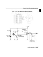
PLC can exchange data with at least other PLCs of the same make. Figure 0.9 shows a PLC as it might be
connected for a position-control application: reading digital input sensors, controlling AC motors, and exchanging
information with the operator.
Another advance which made automation possible was the development of the robot. A variation on NC
equipment, the robot is a self-enclosed system of actuators, sensors and controller. Compatibility of robot

components is the robot manufacturer's problem. A robot includes built-in programs allowing the user to "teach"
positions to the arm, and to play-back moves. Robot programming languages are similar to other computer
programming languages, like BASIC. Even the early robots allowed connection of certain types of external sensors
and actuators, so complete work cells could be built around, and controlled by, the robot. Modern robots usually
include communication ports, so that robots can exchange information with other computerized equipment with
similar communication ports.
The third advance was the introduction, by IBM, of the personal computer (PC). (IBM's use of the name "PC"
forced the suppliers of programmable controllers to start calling their "PC"s by another name. hence the "PLC.")
IBM's PC included a feature then called open architecture. What this meant was that inside the computer box was a
computer on a single "mother" circuit-board and several slots on this "motherboard." Each slot is a standard
connector into a standard bus (set of conductors controlled by the computer). This architecture was called "open"
because IBM made information available so that other manufacturers could design circuit boards that could he
plugged into the bus. IBM also provided information on the operation of the motherboard so that others could write
IBM PC programs to use the new circuit boards. IBM undertook to avoid changes to the motherboard that would
obsolete the important bus and motherboard standards. Boards could be designed and software written to interface
the IBM PC to sensors, actuators, NC equipment, PLCs, robots, or other computers, without IBM having to do the
design or programming. Coupled with IBM's perceived dependability, this "open architecture" provided the
standard that was missing. Now computerization of the factory floor could proceed.


Fig. 0.8 (a) A programmable controller; (b) installation of I/O module on bus unit. (Photographs by
permission, Westinghouse Electric Corporation/ Electrical Components Division, Pittsburgh, Pennsylvania.)
Chapter 0. Introducation
0.5.1 Interfacing of Controllers to Controllers
Standards for what form the signals should take for communication between computers are still largely missing.
The PLC, robot, and computer manufacturers have each developed their own standards, hut one supplier's
equipment can't communicate very easily with another's.
Most suppliers do, at least, build their standards around a very basic set of standards which dates back several
decades to the days of teletype machines: the RS 232 standard. Because of the acceptance of RS 232, a determined
user can usually write controller programs which exchange simple messages with each other.

The International Standards Organization (ISO) is working to develop a common communication standard, known
as the OSI (Open Systems Interconnectivity) model. Several commercial computer networks are already available,
many using the agreed-on parts of the OSI model. Manufacturer's Automation Protocol (MAP) and Technical and
Office Protocol (TOP) are the best-known of these.
Despite the recognition that common standards are needed to be recognized, the immediate need for
communications is leading to the growth of immediately available proprietary standards.


Fig. 0.9 A PLC in a position control application. (Illustration by permission, OMRON Canada Inc.,
Scarborough, Ontario, Canada.)
Chapter 0. Introduction

Several large PLC manufacturers sell proprietary local area networks and actively encourage others to join them in
using those standards. Simultaneous growth of proprietary office local area network suppliers means that
interconnecting the plant to the manufacturing office is becoming another problem area. One promising aspect of
the growth of giants in the local area network field is that the giants recognize the need for easy-to-use interfaces
between their systems, and have the money to develop them.
0.5.2 Interfacing of Controllers to Other Components
One area in which development of standards is not as great a problem is the connection of sensors and actuators to
controllers. This area is a less severe problem because electrical actuators have been available for so long that
several standards are effectively in force.
The 24 volt DC solenoid-actuated valve is an example. 240 volt three phase AC is another standard, dictated by
power supply utility companies. Sensor suppliers, more recent arrivals, have simply adopted those standards most
appropriate to their target market.
Lack of a single standard is still an inconvenience. Signal conditioning is often required so that incompatible
components and controllers can be interconnected. The size of the problem can be reduced by the user by selecting
components with similar power requirements and control signal characteristics, if possible. Another option is using
a PLC as the controller, and selecting a PLC which offers I/O modules for all the different sensors and actuators to
be used.
The user could also consider employing popular "open architecture" computers that can be retrofitted with

interfacing circuit cards available from several sources; however, programming the control program to use those
interface cards requires some skill. Another alternative is buying or building signal conditioning interface circuits
to do signal modification such as:
● cleaning noisy electrical signals
● isolating high power signals from low power signals " amplification (or de-amplification) of current or
voltage levels
● converting analog signals to/from digital numbers
● converting DC signals to/from AC signals
● converting electrical signals to/from non-electrical signals

0.6 SUMMARY
Automation can be used to reduce manufacturing costs. It is more appropriately used to improve quality and make
it more consistent.
This chapter looked at a Computer Integrated Manufacturing environment, so that users of this book will be able to
Chapter 0. Introduction
anticipate the potential third step in the simplify-automate-integrate process as they design individual islands of
automated manufacturing.
An automated process must be able to measure and control its output. "Closed loop control" is the term used for a
self-controlled automated process. A complete closed loop control system requires an actuator (perhaps several
working together), which responds to signals from a controller, and at least one sensor that the controller uses to
ensure that the manufacturing process is proceeding as it should. Most controlled automation processes use several
sensors, to detect incoming materials and workplace environmental conditions, as well as to measure and verify the
process's output.
Digital computers are used in modem soft automation systems, replacing hard automation controllers. Custom-built
analog controllers, traditionally used for process control applications, are examples of "hard" automation. The main
advantages to be reaped by using digital control are in the area of increased flexibility. Digital controllers,
including PLCs, can be programmed to respond to more conditions, in more ways, and can be reprogrammed more
easily than hard automation. The initial system design and building steps are easier, too, because off-the-shelf
components can be used.
Numerical controlled (NC) machining components, analog process controllers, and mechanical and electrical

sequencers have been available for quite a while, but the development of programmable controllers (PLCs), robots,
and open-architecture computers really made automation accessible to the average industrial user. Signal
conditioning is still required to get some components to work with other components. While computerized
equipment can be programmed to communicate with each other, standardization in communication between
computerized equipment is not fully realized yet.

End
| Contents | Chapter 0 | Chapter 1 | Chapter 2 | Chapter 3 | Chapter
4 | Chapter 5 | Chapter 6 | Chapter 7 | Chapter 8 | Chapter 9 |
Chapter 10 | Chapter 11 | Chapter 12 |
Chapter 1. Sensors
Chapter 1. SENSORS
Good sensors are essential in any automated system. Computer Integrated Manufacturing (CIM) is
possible only if comput to end. Some sensors detect only part presence. Other sensors, bar code readers,
for example, help to track materials, tooling, and products as they enter, go through, and leave CIM
environments. In fact, every automated manufacturing operation should include a sensor to ensure it is
working correctly.

1.1 QUALITY OF SENSORS
The best sensor for any job is one that has sufficient quality for the job, has adequate durability, yet isn't
any more expensive than the job requires. Spec sheets (short for "specification sheets") use many terms
to describe how good sensors are. The following section discusses what these terms mean.

1.1.1 Range and Span
The range, or "span," of a sensor describes the limits of the measured variable that a sensor is capable of
sensing. A temperature transducer must have an output (e.g., electric current) that is proportional to
temperature. There are upper and lower limits on the temperature range at which this relationship is
reasonably proportional. Figure 1.1 shows the concept of span in describing the usefulness of a resistance-
type temperature sensor. Current flow through the sensor varies with temperature between t
1 and t4, but is

only reasonably proportional to temperatures between t
2
and t
3
To be able to claim reasonable
proportionality, the sensor's supplier would actually quote the more restrictive temperature span of from
t
2
to t
3
.

1.1.2 Error
The error between the ideal and the actual output of a sensor can be due to many sources. The types of
error can be described as resolution error, linearity error, and repeatability error.

Chapter 1. Sensors
Fig. 1.1 Range and linearity error in a temperature sensor

1.1.3 Resolution
The resolution value quoted for a sensor is the largest change in measured value that will not result in a
change in the sensor's output. Put more simply, the measured value can change by the amount quoted as
resolution, without the sensor's output changing. There are several reasons why resolution error may
occur. Figure 1.2 demonstrates resolution error due to hysteresis. Small changes in measured value are
insufficient to cause a change in the output of the analog sensor. Figure 1.3 demonstrates resolution error
in a sensor with digital output. The digital sensor can output 256 different values for temperature. The
sensor's total span must be divided into 256 temperature ranges. Temperature changes within one of these
subranges cannot be detected. Sensors with more range often have less resolution.

Chapter 1. Sensors

Fig. 1.2 Hysteresis and resolution in a temperature sensor

Fig.1. 3 Resolution in a digital temperature sensor output numbers representing temperature step
input (temperature)

1.1.3 Repeatability
Values quote for a sensor's repeatability indicate the range of output values that the user can expect when
the sensor measures the same input values several times. The temperature sensor in Figure 1.2, for
example, might output any value from a voltage value slightly higher than V
1
to a value slightly lower
when the actual temperature is at temp 1. Repeatability does not necessarily mean that the output value
accurately represents the sensed condition! Looseness in mechanical linkages are one source of
Chapter 1. Sensors
repeatability error.

1.1.4 Linearity
The ideal transducer is one that has an output exactly proportional to the variable it measures (within the
sensor's quoted range). No transducer's output is perfectly proportional to its input, however, so the sensor
user must be aware of the extent of the failure to be linear. Linearity is often quoted on spec sheets as a +/-
value for the sensor's output signal. Figure 1.4 demonstrates what a linearity specification of +/- 0.5 volts
for a pressure sensor means.

1.2 SWITCHES AND TRANSDUCERS
Some simple sensors can distinguish between only two different states of the measured variable. Such
sensors are called switches. Other sensors, called transducers, provide output signals (usually electrical)
that vary in strength with the condition being sensed. Figure 1.5 shows the difference in outputs of a
switch and a transducer to the same sensed condition.

Fig.1. 4 Non-linearity in a pressure sensor

Chapter 1. Sensors
1.2.1 Switches
The most commonly-used sensor in industry is still the simple, inexpensive limit switch, shown in Figure
1.6. These switches are intended to be used as presence sensors. When an object pushes against them,
lever action forces internal connections to be changed.
Most switches can be wired as either normally open (NO) or normally closed (NC). If a force is
required to hold them at the other state, then they are momentary contact switches. Switches that hold
their most recent state after the force is removed are called detent switches.
Most switches are single throw (ST) switches, with only two positions. Switches that have a center
position, but can be forced in either direction, to either of two sets of contacts, are called double throw
(DT). Most double throw switches do not close any circuit when in the center (normal) position, so the
letters "co," for center off, may appear on the spec sheet.

Fig. 1.5 Switch output versus transducer output (switch without hysteresis)

Switches that change more than one set of contacts ("poles") with a single "throw" are also available.
These switches are called double pole (DP), triple pole (TP), etc., instead of the more common single
pole (SP).
In switches designed for high current applications, the contacts are made crude but robust, so that arcing
does not destroy them. For small current applications, typical in computer controlled applications, it is
advisable to use sealed switches with plated contacts to prevent even a slight corrosion layer or oil film
that may radically affect current flow. Small limit switches are often called microswitches.
Any switch with sprung contacts will allow the contacts to bounce when they change position. A
controller monitoring the switch would detect the switch opening and closing rapidly for a short time.
Arcing of current across contacts that are not yet quite touching looks like contact bouncing, too. Where
the control system is sensitive to this condition, two solutions are possible without abandoning limit
Chapter 1. Sensors
switches.

Fig.1.6 Limit switches. (Photograph by permission, Allen-Bradley Canada Ltd., A Rockwell
International Company)

One solution, used in computer keyboards to prevent single keystrokes from being mistaken as multiple
keystrokes, is to include a keystroke-recognition program that refuses to recognize two sequential "on"
states from a single key unless there is a significant time delay between them. This method of
debouncing a switch can be written into machine-language control programs.
Another solution to the bounce problem, and to the contact conductivity problem, is to select one of the
growing number of non-contact limit switches. These limit switches are not actually limit switches but
are supplied in the same casings as traditional limit switches and can be used interchangeably with old
style limit switches. Objects must still press against the lever to change the state of these switches, but
what happens inside is different.
Chapter 1. Sensors
The most common non-contact limit switch, shown in Figure 1.7, is the Hall effect switch. Inside this
switch, the lever moves a magnet toward a Hall effect sensor. An electric current continuously passes
lengthwise through the Hall effect sensor. As the magnet approaches the sensor, this current is forced
toward one side of the sensor. Contacts at the sides of the Hall effect sensor detect that the current is now
concentrated at one side; there is now a voltage across the contacts. This voltage opens or closes a
semiconductor switch. Although the switch operation appears complex, the integrated circuit is
inexpensive.

1.2.2 Non-Contact Presence Sensors (Proximity Sensors)
The limit switches discussed in the previous section are "contact" presence sensors, in that they have to be
touched by an object for that object's presence to be sensed. Contact sensors are often avoided in
automated systems because wherever parts touch there is wear and a potential for eventual failure of the
sensor. Automated systems are increasingly being designed with non-contact sensors. The three most
common types of non-contact sensors in use today are the inductive proximity sensor, the capacitive
proximity sensor, and the optical proximity sensor. All of these sensors are actually transducers, but
they include control circuitry that allows them to be used as switches. The circuitry changes an internal

switch when the transducer output reaches a certain value.

Fig.1. 7 Hall effect limit switches
Chapter 1. Sensors


Fig. 1.8 Inductive proximity sensors. (Photograph by permission, Balluff Inc., Florence, Kentucky.)

The inductive proximity sensor is the most widely used non-contact sensor due to its small size,
robustness, and low cost. This type of sensor can detect only the presence of electrically conductive
materials. Figure 1.8 demonstrates its operating principle.
The supply DC is used to generate AC in an internal coil, which in turn causes an alternating magnetic
field. If no conductive materials are near the face of the sensor, the only impedance to the internal AC is
due to the inductance of the coil. If, however, a conductive material enters the changing magnetic field,
eddy currents are generated in that conductive material, and there is a resultant increase in the impedance
Chapter 1. Sensors
to the AC in the proximity sensor. A current sensor, also built into the proximity sensor, detects when
there is a drop in the internal AC current due to increased impedance. The current sensor controls a
switch providing the output.
Capacitive proximity sensors sense "target" objects due to the target's ability to be electrically charged.
Since even non-conductors can hold charges, this means that just about any object can be detected with
this type of sensor. Figure 1.9 demonstrates the principle of capacitive proximity sensing.
Inside the sensor is a circuit that uses the supplied DC power to generate AC, to measure the current in
the internal AC circuit, and to switch the output circuit when the amount of AC current changes. Unlike
the inductive sensor, however, the AC does not drive a coil, but instead tries to charge a capacitor.
Remember that capacitors can hold a charge because, when one plate is charged positively, negative
charges are attracted into the other plate, thus allowing even more positive charges to be introduced into
the first plate. Unless both plates are present and close to each other, it is very difficult to cause either
plate to take on very much charge. Only one of the required two capacitor plates is actually built into the
capacitive sensor! The AC can move current into and out of this plate only if there is another plate nearby

that can hold the opposite charge. The target being sensed acts as the other plate. If this object is near
enough to the face of the capacitive sensor to be affected by the charge in the sensor's internal capacitor
plate, it will respond by becoming oppositely charged near the sensor, and the sensor will then be able to
move significant current into and out of its internal plate.
Optical proximity sensors generally cost more than inductive proximity sensors, and about the same as
capacitive sensors. They are widely used in automated systems because they have been available longer
and because some can fit into small locations. These sensors are more commonly known as light beam
sensors of the thru-beam type or of the retroreflective type. Both sensor types are shown in Figure 1.10.
A complete optical proximity sensor includes a light source, and a sensor that detects the light.

Fig.1. 9 Capacitive proximity sensors.
The light source is supplied because it is usually critical that the light be "tailored" for the light sensor