teletraffic engineering handbook

ITU–D
Study Group 2
Question 16/2
Handbook
“TELETRAFFIC ENGINEERING”
Geneva, January 2005
ii
iii
PREFACE
This first edition of the Teletraffic Engineering Handbook has been worked out as a joint
venture between the
• ITU – International Telecommunication Union
<>, and the:
• ITC – International Teletraffic Congress
<>.
The handbook covers the basic theory of teletraffic engineering. The mathematical back-
ground required is elementary probability theory. The purpose of the handbook is to enable
engineers to understand ITU–T recommendations on traffic engineering, evaluate tools and
methods, and keep up-to-date with new practices. The book includes the following parts:
• Introduction: Chapter 1 – 2,
• Mathematical background: Chapter 3 – 6,
• Telecommunication loss models: Chapter 7 – 11,
• Data communication delay models: Chapter 12 – 14,
• Measurements: Chapter 15.
The purpose of the book is twofold: to serve both as a handbook and as a textbook. Thus
the reader should, for example, be able to study chapters on loss models without studying
the chapters on the mathematical background first.
The handbook is based on many years of experience in teaching the subject at the Tech-
nical University of Denmark and from ITU training courses in developing countries by
the editor Villy B. Iversen. ITU-T Study Group 2 (Working Party 3/2) has reviewed
Recommendations on traffic engineering. Many engineers from the international teletraf-

fic community and students have contributed with ideas to the presentation. Supporting
material, such as software, exercises, advanced material, and case studies, is available at
< where comments and ideas will also be appreci-
ated.
The handbook was initiated by the International Teletraffic Congress (ITC), Committee 3
(Developing countries and ITU matters), reviewed and adopted by ITU-D Study Group 2
in 2001. The Telecommunication Development Bureau thanks the International Teletraffic
Congress, all Member States, Sector Members and experts, who contributed to this publica-
tion.
Hamadoun I. Tour´e
Director
Telecommunication Development Bureau
International Telecommunication Union
iv
v
Notations
a Carried traffic per source or per channel
A Offered traffic = A
o
A
c
Carried traffic = Y
A

Lost traffic
B Call congestion
B Burstiness
c Constant
C Traffic congestion = load congestion
C

n
Catalan’s number
d Slot size in multi-rate traffic
D Probability of delay or
Deterministic arrival or service process
E Time congestion
E
1,n
(A) = E
1
Erlang’s B–formula = Erlang’s 1. formula
E
2,n
(A) = E
2
Erlang’s C–formula = Erlang’s 2. formula
F Improvement function
g Number of groups
h Constant time interval or service time
H(k) Palm–Jacobæus’ formula
I Inverse time congestion I = 1/E
J
ν
(z) Modified Bessel function of order ν
k Accessibility = hunting capacity
Maximum number of customers in a queueing system
K Number of links in a telecommuncation network or
number of nodes in a queueing network
L Mean queue length
L

kø
Mean queue length when the queue is greater than zero
L Random variable for queue length
m Mean value (average) = m
1
m
i
i’th (non-central) moment
m

i
i’th centrale moment
m
r
Mean residual life time
M Poisson arrival process
n Number of servers (channels)
N Number of traffic streams or traffic types
p(i) State probabilities, time averages
p{i, t |j, t
0
} Probability for state i at time t given state j at time t
0
vi
P (i) Cumulated state probabilities P (i) =

i
x=−∞
p(x)
q(i) Relative (non normalised) state probabilities

Q(i) Cumulated values of q(i): Q(i) =

i
x=−∞
q(x)
Q Normalisation constant
r Reservation parameter (trunk reservation)
R Mean response time
s Mean service time
S Number of traffic sources
t Time instant
T Random variable for time instant
U Load function
v Variance
V Virtual waiting time
w Mean waiting time for delayed customers
W Mean waiting time for all customers
W Random variable for waiting time
x Variable
X Random variable
y Arrival rate. Poisson process: y = λ
Y Carried traffic
Z Peakedness
α Offered traffic per source
β Offered traffic per idle source
γ Arrival rate for an idle source
ε Palm’s form factor
ϑ Lagrange-multiplicator
κ
i

i’th cumulant
λ Arrival rate of a Poisson process
Λ Total arrival rate to a system
µ Service rate, inverse mean service time
π(i) State probabilities, arriving customer mean values
ψ(i) State probabilities, departing customer mean values
 Service ratio
σ
2
Variance, σ = standard deviation
τ Time-out constant or constant time-interval
Contents
1 Introduction to Teletraffic Engineering 1
1.1 Modelling of telecommunication systems . . . . . . . . . . . . . . . . . . . . . 2
1.1.1 System structure . . . . . . . . . . . . . . . . . . . . . . . . . . . . . . 3
1.1.2 The operational strategy . . . . . . . . . . . . . . . . . . . . . . . . . 3
1.1.3 Statistical properties of traffic . . . . . . . . . . . . . . . . . . . . . . . 3
1.1.4 Models . . . . . . . . . . . . . . . . . . . . . . . . . . . . . . . . . . . 5
1.2 Conventional telephone systems . . . . . . . . . . . . . . . . . . . . . . . . . . 5
1.2.1 System structure . . . . . . . . . . . . . . . . . . . . . . . . . . . . . . 6
1.2.2 User behaviour . . . . . . . . . . . . . . . . . . . . . . . . . . . . . . . 7
1.2.3 Operation strategy . . . . . . . . . . . . . . . . . . . . . . . . . . . . . 8
1.3 Communication networks . . . . . . . . . . . . . . . . . . . . . . . . . . . . . 9
1.3.1 The telephone network . . . . . . . . . . . . . . . . . . . . . . . . . . . 9
1.3.2 Data networks . . . . . . . . . . . . . . . . . . . . . . . . . . . . . . . 11
1.3.3 Local Area Networks (LAN) . . . . . . . . . . . . . . . . . . . . . . . 12
1.4 Mobile communication systems . . . . . . . . . . . . . . . . . . . . . . . . . . 13
1.4.1 Cellular systems . . . . . . . . . . . . . . . . . . . . . . . . . . . . . . 13
1.5 ITU recommendations on traffic engineering . . . . . . . . . . . . . . . . . . . 16
1.5.1 Traffic engineering in the ITU . . . . . . . . . . . . . . . . . . . . . . . 16

1.5.2 Traffic demand characterisation . . . . . . . . . . . . . . . . . . . . . . 17
1.5.3 Grade of Service objectives . . . . . . . . . . . . . . . . . . . . . . . . 23
1.5.4 Traffic controls and dimensioning . . . . . . . . . . . . . . . . . . . . . 28
1.5.5 Performance monitoring . . . . . . . . . . . . . . . . . . . . . . . . . . 35
1.5.6 Other recommendations . . . . . . . . . . . . . . . . . . . . . . . . . . 36
1.5.7 Work program for the Study Period 2001–2004 . . . . . . . . . . . . . 37
1.5.8 Conclusions . . . . . . . . . . . . . . . . . . . . . . . . . . . . . . . . . 38
2 Traffic concepts and grade of service 39
2.1 Concept of traffic and traffic unit [erlang] . . . . . . . . . . . . . . . . . . . . 39
vii
viii CONTENTS
2.2 Traffic variations and the concept busy hour . . . . . . . . . . . . . . . . . . . 42
2.3 The blocking concept . . . . . . . . . . . . . . . . . . . . . . . . . . . . . . . 45
2.4 Traffic generation and subscribers reaction . . . . . . . . . . . . . . . . . . . . 48
2.5 Introduction to Grade-of-Service = GoS . . . . . . . . . . . . . . . . . . . . . 55
2.5.1 Comparison of GoS and QoS . . . . . . . . . . . . . . . . . . . . . . . 56
2.5.2 Special features of QoS . . . . . . . . . . . . . . . . . . . . . . . . . . 57
2.5.3 Network performance . . . . . . . . . . . . . . . . . . . . . . . . . . . 57
2.5.4 Reference configurations . . . . . . . . . . . . . . . . . . . . . . . . . . 58
3 Probability Theory and Statistics 61
3.1 Distribution functions . . . . . . . . . . . . . . . . . . . . . . . . . . . . . . . 61
3.1.1 Characterisation of distributions . . . . . . . . . . . . . . . . . . . . . 62
3.1.2 Residual lifetime . . . . . . . . . . . . . . . . . . . . . . . . . . . . . . 64
3.1.3 Load from holding times of duration less than x . . . . . . . . . . . . . 67
3.1.4 Forward recurrence time . . . . . . . . . . . . . . . . . . . . . . . . . . 68
3.1.5 Distribution of the j’th largest of k random variables . . . . . . . . . . 69
3.2 Combination of random variables . . . . . . . . . . . . . . . . . . . . . . . . . 70
3.2.1 Random variables in series . . . . . . . . . . . . . . . . . . . . . . . . 70
3.2.2 Random variables in parallel . . . . . . . . . . . . . . . . . . . . . . . 71
3.3 Stochastic sum . . . . . . . . . . . . . . . . . . . . . . . . . . . . . . . . . . . 72

4 Time Interval D istributions 75
4.1 Exponential distribution . . . . . . . . . . . . . . . . . . . . . . . . . . . . . . 75
4.1.1 Minimum of k exponentially distributed random variables . . . . . . . 77
4.1.2 Combination of exponential distributions . . . . . . . . . . . . . . . . 78
4.2 Steep distributions . . . . . . . . . . . . . . . . . . . . . . . . . . . . . . . . . 78
4.3 Flat distributions . . . . . . . . . . . . . . . . . . . . . . . . . . . . . . . . . . 80
4.3.1 Hyper-exponential distribution . . . . . . . . . . . . . . . . . . . . . . 81
4.4 Cox distributions . . . . . . . . . . . . . . . . . . . . . . . . . . . . . . . . . . 82
4.4.1 Polynomial trial . . . . . . . . . . . . . . . . . . . . . . . . . . . . . . 86
4.4.2 Decomposition principles . . . . . . . . . . . . . . . . . . . . . . . . . 86
4.4.3 Importance of Cox distribution . . . . . . . . . . . . . . . . . . . . . . 88
4.5 Other time distributions . . . . . . . . . . . . . . . . . . . . . . . . . . . . . . 89
4.6 Observations of life-time distribution . . . . . . . . . . . . . . . . . . . . . . . 90
5 Arrival Processes 93
5.1 Description of point processes . . . . . . . . . . . . . . . . . . . . . . . . . . . 93
CONTENTS ix
5.1.1 Basic properties of number representation . . . . . . . . . . . . . . . . 95
5.1.2 Basic properties of interval representation . . . . . . . . . . . . . . . . 96
5.2 Characteristics of point process . . . . . . . . . . . . . . . . . . . . . . . . . . 97
5.2.1 Stationarity (Time homogeneity) . . . . . . . . . . . . . . . . . . . . . 98
5.2.2 Independence . . . . . . . . . . . . . . . . . . . . . . . . . . . . . . . . 98
5.2.3 Simple point process . . . . . . . . . . . . . . . . . . . . . . . . . . . . 99
5.3 Little’s theorem . . . . . . . . . . . . . . . . . . . . . . . . . . . . . . . . . . 99
6 The Poisson process 103
6.1 Characteristics of the Poisson process . . . . . . . . . . . . . . . . . . . . . . 103
6.2 Distributions of the Poisson process . . . . . . . . . . . . . . . . . . . . . . . 104
6.2.1 Exponential distribution . . . . . . . . . . . . . . . . . . . . . . . . . . 105
6.2.2 Erlang–k distribution . . . . . . . . . . . . . . . . . . . . . . . . . . . 107
6.2.3 Poisson distribution . . . . . . . . . . . . . . . . . . . . . . . . . . . . 108
6.2.4 Static derivation of the distributions of the Poisson process . . . . . . 111

6.3 Properties of the Poisson process . . . . . . . . . . . . . . . . . . . . . . . . . 112
6.3.1 Palm’s theorem . . . . . . . . . . . . . . . . . . . . . . . . . . . . . . . 112
6.3.2 Raikov’s theorem (Decomposition theorem) . . . . . . . . . . . . . . . 115
6.3.3 Uniform distribution – a conditional property . . . . . . . . . . . . . . 115
6.4 Generalisation of the stationary Poisson process . . . . . . . . . . . . . . . . . 115
6.4.1 Interrupted Poisson process (IPP) . . . . . . . . . . . . . . . . . . . . 117
7 Erlang’s loss system and B–formula 119
7.1 Introduction . . . . . . . . . . . . . . . . . . . . . . . . . . . . . . . . . . . . 119
7.2 Poisson distribution . . . . . . . . . . . . . . . . . . . . . . . . . . . . . . . . 120
7.2.1 State transition diagram . . . . . . . . . . . . . . . . . . . . . . . . . . 120
7.2.2 Derivation of state probabilities . . . . . . . . . . . . . . . . . . . . . . 122
7.2.3 Traffic characteristics of the Poisson distribution . . . . . . . . . . . . 123
7.3 Truncated Poisson distribution . . . . . . . . . . . . . . . . . . . . . . . . . . 124
7.3.1 State probabilities . . . . . . . . . . . . . . . . . . . . . . . . . . . . . 125
7.3.2 Traffic characteristics of Erlang’s B-formula . . . . . . . . . . . . . . . 125
7.3.3 Generalisations of Erlang’s B-formula . . . . . . . . . . . . . . . . . . 128
7.4 Standard procedures for state transition diagrams . . . . . . . . . . . . . . . . 128
7.4.1 Recursion formula . . . . . . . . . . . . . . . . . . . . . . . . . . . . . 132
7.5 Evaluation of Erlang’s B-formula . . . . . . . . . . . . . . . . . . . . . . . . . 134
7.6 Principles of dimensioning . . . . . . . . . . . . . . . . . . . . . . . . . . . . . 136
x CONTENTS
7.6.1 Dimensioning with fixed blocking probability . . . . . . . . . . . . . . 136
7.6.2 Improvement principle (Moe’s principle) . . . . . . . . . . . . . . . . . 137
8 Loss systems with full accessibility 141
8.1 Introduction . . . . . . . . . . . . . . . . . . . . . . . . . . . . . . . . . . . . 142
8.2 Binomial Distribution . . . . . . . . . . . . . . . . . . . . . . . . . . . . . . . 143
8.2.1 Equilibrium equations . . . . . . . . . . . . . . . . . . . . . . . . . . . 144
8.2.2 Traffic characteristics of Binomial traffic . . . . . . . . . . . . . . . . . 146
8.3 Engset distribution . . . . . . . . . . . . . . . . . . . . . . . . . . . . . . . . . 148
8.3.1 State probabilities . . . . . . . . . . . . . . . . . . . . . . . . . . . . . 149

8.3.2 Traffic characteristics of Engset traffic . . . . . . . . . . . . . . . . . . 149
8.4 Evaluation of Engset’s formula . . . . . . . . . . . . . . . . . . . . . . . . . . 153
8.4.1 Recursion formula on n . . . . . . . . . . . . . . . . . . . . . . . . . . 153
8.4.2 Recursion formula on S . . . . . . . . . . . . . . . . . . . . . . . . . . 154
8.4.3 Recursion formula on both n and S . . . . . . . . . . . . . . . . . . . . 155
8.5 Relationships between E, B, and C . . . . . . . . . . . . . . . . . . . . . . . . 155
8.6 Pascal Distribution (Negative Binomial) . . . . . . . . . . . . . . . . . . . . . 157
8.7 Truncated Pascal distribution . . . . . . . . . . . . . . . . . . . . . . . . . . . 158
9 Overflow theory 163
9.1 Overflow theory . . . . . . . . . . . . . . . . . . . . . . . . . . . . . . . . . . 164
9.1.1 State probability of overflow systems . . . . . . . . . . . . . . . . . . . 165
9.2 Equivalent Random Traffic method . . . . . . . . . . . . . . . . . . . . . . . . 167
9.2.1 Preliminary analysis . . . . . . . . . . . . . . . . . . . . . . . . . . . . 168
9.2.2 Numerical aspects . . . . . . . . . . . . . . . . . . . . . . . . . . . . . 169
9.2.3 Parcel blocking probabilities . . . . . . . . . . . . . . . . . . . . . . . . 170
9.3 Fredericks & Hayward’s method . . . . . . . . . . . . . . . . . . . . . . . . . 172
9.3.1 Traffic splitting . . . . . . . . . . . . . . . . . . . . . . . . . . . . . . . 173
9.4 Other methods based on state space . . . . . . . . . . . . . . . . . . . . . . . 175
9.4.1 BPP traffic models . . . . . . . . . . . . . . . . . . . . . . . . . . . . . 175
9.4.2 Sanders’ method . . . . . . . . . . . . . . . . . . . . . . . . . . . . . . 175
9.4.3 Berkeley’s method . . . . . . . . . . . . . . . . . . . . . . . . . . . . . 176
9.5 Methods based on arrival processes . . . . . . . . . . . . . . . . . . . . . . . . 177
9.5.1 Interrupted Poisson Process . . . . . . . . . . . . . . . . . . . . . . . . 177
9.5.2 Cox–2 arrival process . . . . . . . . . . . . . . . . . . . . . . . . . . . 178
10 Multi-Dimensional Loss Systems 181
CONTENTS xi
10.1 Multi-dimensional Erlang-B formula . . . . . . . . . . . . . . . . . . . . . . . 181
10.2 Reversible Markov processes . . . . . . . . . . . . . . . . . . . . . . . . . . . . 185
10.3 Multi-Dimensional Loss Systems . . . . . . . . . . . . . . . . . . . . . . . . . 187
10.3.1 Class limitation . . . . . . . . . . . . . . . . . . . . . . . . . . . . . . 187

10.3.2 Generalised traffic processes . . . . . . . . . . . . . . . . . . . . . . . . 187
10.3.3 Multi-slot traffic . . . . . . . . . . . . . . . . . . . . . . . . . . . . . . 188
10.4 Convolution Algorithm for loss systems . . . . . . . . . . . . . . . . . . . . . 192
10.4.1 The algorithm . . . . . . . . . . . . . . . . . . . . . . . . . . . . . . . 193
10.4.2 Other algorithms . . . . . . . . . . . . . . . . . . . . . . . . . . . . . . 199
11 Dimensioning of telecom networks 205
11.1 Traffic matrices . . . . . . . . . . . . . . . . . . . . . . . . . . . . . . . . . . . 205
11.1.1 Kruithof’s double factor method . . . . . . . . . . . . . . . . . . . . . 206
11.2 Topologies . . . . . . . . . . . . . . . . . . . . . . . . . . . . . . . . . . . . . 209
11.3 Routing principles . . . . . . . . . . . . . . . . . . . . . . . . . . . . . . . . . 209
11.4 Approximate end-to-end calculations methods . . . . . . . . . . . . . . . . . . 209
11.4.1 Fix-point method . . . . . . . . . . . . . . . . . . . . . . . . . . . . . 209
11.5 Exact end-to-end calculation methods . . . . . . . . . . . . . . . . . . . . . . 210
11.5.1 Convolution algorithm . . . . . . . . . . . . . . . . . . . . . . . . . . . 210
11.6 Load control and service protection . . . . . . . . . . . . . . . . . . . . . . . . 210
11.6.1 Trunk reservation . . . . . . . . . . . . . . . . . . . . . . . . . . . . . 211
11.6.2 Virtual channel protection . . . . . . . . . . . . . . . . . . . . . . . . . 212
11.7 Moe’s principle . . . . . . . . . . . . . . . . . . . . . . . . . . . . . . . . . . . 212
11.7.1 Balancing marginal costs . . . . . . . . . . . . . . . . . . . . . . . . . 213
11.7.2 Optimum carried traffic . . . . . . . . . . . . . . . . . . . . . . . . . . 214
12 Delay Systems 217
12.1 Erlang’s delay system M/M/n . . . . . . . . . . . . . . . . . . . . . . . . . . . 217
12.2 Traffic characteristics of delay systems . . . . . . . . . . . . . . . . . . . . . . 219
12.2.1 Erlang’s C-formula . . . . . . . . . . . . . . . . . . . . . . . . . . . . . 219
12.2.2 Numerical evaluation . . . . . . . . . . . . . . . . . . . . . . . . . . . 220
12.2.3 Mean queue lengths . . . . . . . . . . . . . . . . . . . . . . . . . . . . 221
12.2.4 Mean waiting times . . . . . . . . . . . . . . . . . . . . . . . . . . . . 223
12.2.5 Improvement functions for M/M/n . . . . . . . . . . . . . . . . . . . . 225
12.3 Moe’s principle for delay systems . . . . . . . . . . . . . . . . . . . . . . . . . 225
12.4 Waiting time distribution for M/M/n, FCFS . . . . . . . . . . . . . . . . . . 227

xii CONTENTS
12.4.1 Response time with a single server . . . . . . . . . . . . . . . . . . . . 229
12.5 Palm’s machine repair model . . . . . . . . . . . . . . . . . . . . . . . . . . . 230
12.5.1 Terminal systems . . . . . . . . . . . . . . . . . . . . . . . . . . . . . . 231
12.5.2 State probabilities – single server . . . . . . . . . . . . . . . . . . . . . 232
12.5.3 Terminal states and traffic characteristics . . . . . . . . . . . . . . . . 235
12.5.4 Machine–repair model with n servers . . . . . . . . . . . . . . . . . . . 238
12.6 Optimising the machine-repair model . . . . . . . . . . . . . . . . . . . . . . . 240
13 Applied Queueing Theory 245
13.1 Classification of queueing models . . . . . . . . . . . . . . . . . . . . . . . . . 245
13.1.1 Description of traffic and structure . . . . . . . . . . . . . . . . . . . . 245
13.1.2 Queueing strategy: disciplines and organisation . . . . . . . . . . . . . 246
13.1.3 Priority of customers . . . . . . . . . . . . . . . . . . . . . . . . . . . . 248
13.2 General results in the queueing theory . . . . . . . . . . . . . . . . . . . . . . 249
13.3 Pollaczek-Khintchine’s formula for M/G/1 . . . . . . . . . . . . . . . . . . . . 250
13.3.1 Derivation of Pollaczek-Khintchine’s formula . . . . . . . . . . . . . . 250
13.3.2 Busy period for M/G/1 . . . . . . . . . . . . . . . . . . . . . . . . . . 251
13.3.3 Waiting time for M/G/1 . . . . . . . . . . . . . . . . . . . . . . . . . . 252
13.3.4 Limited queue length: M/G/1/k . . . . . . . . . . . . . . . . . . . . . 253
13.4 Priority queueing systems: M/G/1 . . . . . . . . . . . . . . . . . . . . . . . . 253
13.4.1 Combination of several classes of customers . . . . . . . . . . . . . . . 254
13.4.2 Work conserving queueing disciplines . . . . . . . . . . . . . . . . . . . 255
13.4.3 Non-preemptive queueing discipline . . . . . . . . . . . . . . . . . . . . 257
13.4.4 SJF-queueing discipline . . . . . . . . . . . . . . . . . . . . . . . . . . 259
13.4.5 M/M/n with non-preemptive priority . . . . . . . . . . . . . . . . . . 262
13.4.6 Preemptive-resume queueing discipline . . . . . . . . . . . . . . . . . . 263
13.5 Queueing systems with constant holding times . . . . . . . . . . . . . . . . . 264
13.5.1 Historical remarks on M/D/n . . . . . . . . . . . . . . . . . . . . . . . 264
13.5.2 State probabilities of M/D/1 . . . . . . . . . . . . . . . . . . . . . . . 265
13.5.3 Mean waiting times and busy period of M/D/1 . . . . . . . . . . . . . 266

13.5.4 Waiting time distribution: M/D/1, FCFS . . . . . . . . . . . . . . . . 267
13.5.5 State probabilities: M/D/n . . . . . . . . . . . . . . . . . . . . . . . . 269
13.5.6 Waiting time distribution: M/D/n, FCFS . . . . . . . . . . . . . . . . 269
13.5.7 Erlang-k arrival process: E
k
/D/r . . . . . . . . . . . . . . . . . . . . . 270
13.5.8 Finite queue system: M/D/1/k . . . . . . . . . . . . . . . . . . . . . . 271
13.6 Single server queueing system: GI/G/1 . . . . . . . . . . . . . . . . . . . . . . 272
CONTENTS xiii
13.6.1 General results . . . . . . . . . . . . . . . . . . . . . . . . . . . . . . . 273
13.6.2 State probabilities: GI/M/1 . . . . . . . . . . . . . . . . . . . . . . . . 274
13.6.3 Characteristics of GI/M/1 . . . . . . . . . . . . . . . . . . . . . . . . . 275
13.6.4 Waiting time distribution: GI/M/1, FCFS . . . . . . . . . . . . . . . . 276
13.7 Round Robin and Processor-Sharing . . . . . . . . . . . . . . . . . . . . . . . 277
14 Networks of queues 279
14.1 Introduction to queueing networks . . . . . . . . . . . . . . . . . . . . . . . . 279
14.2 Symmetric queueing systems . . . . . . . . . . . . . . . . . . . . . . . . . . . 280
14.3 Jackson’s theorem . . . . . . . . . . . . . . . . . . . . . . . . . . . . . . . . . 282
14.3.1 Kleinrock’s independence assumption . . . . . . . . . . . . . . . . . . . 285
14.4 Single chain queueing networks . . . . . . . . . . . . . . . . . . . . . . . . . . 285
14.4.1 Convolution algorithm for a closed queueing network . . . . . . . . . . 286
14.4.2 The MVA–algorithm . . . . . . . . . . . . . . . . . . . . . . . . . . . . 290
14.5 BCMP queueing networks . . . . . . . . . . . . . . . . . . . . . . . . . . . . . 293
14.6 Multidimensional queueing networks . . . . . . . . . . . . . . . . . . . . . . . 294
14.6.1 M/M/1 single server queueing system . . . . . . . . . . . . . . . . . . 294
14.6.2 M/M/n queueing system . . . . . . . . . . . . . . . . . . . . . . . . . 297
14.7 Closed queueing networks with multiple chains . . . . . . . . . . . . . . . . . 297
14.7.1 Convolution algorithm . . . . . . . . . . . . . . . . . . . . . . . . . . . 297
14.8 Other algorithms for queueing networks . . . . . . . . . . . . . . . . . . . . . 300
14.9 Complexity . . . . . . . . . . . . . . . . . . . . . . . . . . . . . . . . . . . . . 301

14.10 Optimal capacity allocation . . . . . . . . . . . . . . . . . . . . . . . . . . . . 301
15 Traffic measurements 305
15.1 Measuring principles and methods . . . . . . . . . . . . . . . . . . . . . . . . 306
15.1.1 Continuous measurements . . . . . . . . . . . . . . . . . . . . . . . . . 306
15.1.2 Discrete measurements . . . . . . . . . . . . . . . . . . . . . . . . . . . 307
15.2 Theory of sampling . . . . . . . . . . . . . . . . . . . . . . . . . . . . . . . . . 308
15.3 Continuous measurements in an unlimited period . . . . . . . . . . . . . . . . 310
15.4 Scanning method in an unlimited time period . . . . . . . . . . . . . . . . . . 313
15.5 Numerical example . . . . . . . . . . . . . . . . . . . . . . . . . . . . . . . . . 316
0 CONTENTS
Chapter 1
Introduction to Teletraffic Engineering
Teletraffic theory is defined as the application of probability theory to the solution of problems
concerning planning, p erformance evaluation, operation, and maintenance of telecommuni-
cation systems. More generally, teletraffic theory can be viewed as a discipline of planning
where the tools (stochastic processes, queueing theory and numerical simulation) are taken
from the disciplines of operations research.
The term teletraffic covers all kinds of data communication traffic and telecommunication
traffic. The theory will primarily be illustrated by examples from telephone and data com-
munication systems. The tools developed are, however, independent of the technology and
applicable within other areas such as road traffic, air traffic, manufacturing and assembly
belts, distribution, workshop and storage management, and all kinds of service systems.
The objective of teletraffic theory can be formulated as follows:
to make the traffic measurable in well defined units through mathematical models and
to derive the relationship between grade-of-service and system capacity in such a way
that the theory becomes a tool by which investments can be planned.
The task of teletraffic theory is to design systems as cost effectively as possible with a pre-
defined grade of service when we know the future traffic demand and the capacity of system
elements. Furthermore, it is the task of teletraffic engineering to specify methods for con-
trolling that the actual grade of service is fulfilling the requirements, and also to specify

emergency actions when systems are overloaded or technical faults occur. This requires
methods for forecasting the demand (for instance based on traffic measurements), methods
for calculating the capacity of the systems, and specification of quantitative measures for the
grade of service.
When applying the theory in practice, a series of decision problems concerning both short
term as well as long term arrangements occur.
1
2 CHAPTER 1. INTRODUCTION TO TELETRAFFIC ENGINEERING
Short term decisions include a.o. the determination of the number of circuits in a trunk group,
the number of operators at switching boards, the number of open lanes in the supermarket,
and the allocation of priorities to jobs in a computer system.
Long term decisions include for example decisions concerning the development and extension
of data- and telecommunication networks, the purchase of cable equipment, transmission
systems etc.
The application of the theory in connection with design of new systems can help in comparing
different solutions and thus eliminate non-optimal solutions at an early stage without having
to build up prototypes.
1.1 Modelling of telecommunication systems
For the analysis of a telecommunication system, a model must be set up to describe the
whole (or parts of) the system. This modelling process is fundamental especially for new
applications of the teletraffic theory; it requires knowledge of both the technical system as
well as the mathematical tools and the implementation of the model on a computer. Such a
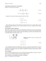
model contains three main elements (Fig. 1.1):
• the system structure,
• the operational strategy, and
• the statistical properties of the traffic.
MACHINE
Deterministic
MAN
Structure

Stochastic User demands
Hardware Software
Strategy
Traffic
Figure 1.1: Telecommunication systems are complex man/machine systems. The task of
teletraffic theory is to configure optimal systems from knowledge of user requirements and
habits.
1.1. MODELLING OF TELECOMMUNICATION SYSTEMS 3
1.1.1 System structure
This part is technically determined and it is in principle possible to obtain any level of details
in the description, e.g. at component level. Reliability aspects are stochastic as errors occur
at random, and they will be dealt with as traffic with a high priority. The system structure
is given by the physical or logical system which is described in manuals in every detail. In
road traffic systems, roads, traffic signals, roundabouts, etc. make up the structure.
1.1.2 The operational strategy
A given physic al sys tem (for instance a roundabout in a road traffic system) can be used
in different ways in order to adapt the traffic system to the demand. In road traffic, it is
implemented with traffic rules and strategies which might be different for the morning and
the evening traffic.
In a computer, this adaption takes place by means of the operation system and by operator
interference. In a telecommunication system, strategies are applied in order to give priority
to call attempts and in order to route the traffic to the destination. In Stored Program
Controlled (SPC) telephone exchanges, the tasks assigned to the central processor are divided
into classes with different priorities. The highest priority is given to accepted calls followed
by new call attempts whereas routine control of equipment has lower priority. The classical
telephone systems used wired logic in order to introduce strategies while in modern systems
it is done by software, enabling more flexible and adaptive strategies.
1.1.3 Statistical properties of traffic
User demands are modelled by statistical properties of the traffic. Only by measurements
on real systems is it possible to validate that the theoretical modelling is in agreement with

reality. This process must necessarily be of an iterative nature (Fig. 1.2). A mathematical
model is build up from a thorough knowledge of the traffic. Properties are then derived from
the model and compared to measured data. If they are not in satisfactory accordance with
each other, a new iteration of the process must take place.
It appears natural to split the description of the traffic prop e rties into stochastic processes for
arrival of call attempts and processes describing service (holding) times. These two processes
are usually assumed to be mutually independent, meaning that the duration of a call is
independent of the time the call arrived. Models also exists for describing the behaviour of
users (subscribers) experiencing blocking, i.e. they are refused service and may make a new
call attempt a little later (repeated call attempts). Fig. 1.3 illustrates the terminology usually
applied in the teletraffic theory.
4 CHAPTER 1. INTRODUCTION TO TELETRAFFIC ENGINEERING
Verification
Model
Observation
Data
Deduction
Figure 1.2: Teletraffic theory is an inductive discipline. From observations of real systems we
establish theoretical models, from which we derive parameters, which can be compared with
corresponding observations from the real system. If there is agreement, the model has been
validated. If not, then we have to elaborate the model further. This scientific way of working
is called the research spiral.
Holding time Idle time
Time
Idle
Busy
Inter-arrival time
Arrival time Departure time
Figure 1.3: Illustration of the terminology applied for a traffic process. Notice the difference
between time intervals and instants of time. We use the terms arrival and call synonymously.

The inter-arrival time, respectively the inter-departure time, are the time intervals between
arrivals, respectively departures.
1.2. CONVENTIONAL TELEPHONE SYSTEMS 5
1.1.4 Models
General requirements to a model are:
1. It must w ithout major difficulty be possible to verify the model and it must be possible
to determine the model parameters from observed data.
2. It must be feasible to apply the model for practical dimensioning.
We are looking for a description of for example the variations observed in the number of
ongoing established calls in a telephone exchange, which vary incessantly due to calls being
established and terminated. Even though common habits of subscribers imply that daily
variations follows a predictable pattern, it is impossible to predict individual call attempts
or duration of individual calls. In the description, it is therefore necessary to use statistical
methods. We say that call attempt events take place according to a stochastic process, and
the inter arrival time between call attempts is described by those probability distributions
which characterise the stochastic process.
An alternative to a mathematical model is a simulation model or a physical model (prototype).
In a computer simulation model it is common to use either collected data directly or to
use artificial data from statistical distributions. It is however, more resource demanding
to work with simulation since the simulation model is not general. Every individual case
must be simulated. The development of a physical prototype is even more time and resource
consuming than a simulation model.
In general mathematical models are the refore preferred but often it is necessary to apply
simulation to develop the mathematical model. Sometimes prototypes are developed for
ultimate testing.
1.2 Conventional telephone systems
This section gives a short description on what happens when a call arrives to a traditional
telephone central. We divide the description into three parts: structure, strategy and traffic.
It is common practice to distinguish between subscriber exchanges (access switches, local
exchanges, LEX) and transit exchanges (TEX) due to the hierarchical structure according

to which most national telephone networks are designed. Subscribers are connected to local
exchanges or to access switches (concentrators), which are connected to local exchanges.
Finally, transit switches are used to interconnect local exchanges or to increase the availability
and reliability.
6 CHAPTER 1. INTRODUCTION TO TELETRAFFIC ENGINEERING
1.2.1 System structure
Here we consider a telephone exchange of the crossbar type. Even though this type is being
taken out of service these years, a description of its functionality gives a good illustration on
the tasks which need to b e solved in a digital exchange. The equipment in a conventional
telephone exchange consists of voice paths and control paths. (Fig. 1.4).
Processor
Register
Subscriber Stage
Group Selector
Junctor
Subscriber
Voice Paths
Control Paths
Processor Processor
Figure 1.4: Fundamental structure of a switching system.
The voice paths are occupied during the whole duration of the call (in average three minutes)
while the control paths only are occupied during the call establishment phase (in the range
0.1 to 1 s). The number of voice paths is therefore considerable larger than the number of
control paths. The voice path is a connection f rom a given inlet (subscriber) to a given outlet.
In a space divided system the voice paths consists of passive component (like relays, diodes
or VLSI circuits). In a time division system the voice paths consist of specific time-slots
within a frame. The control paths are responsible for establishing the connection. Normally,
this happens in a number of stages where each stage is performed by a control device: a
microprocessor, or a register.
Tasks of the control device are:

• Identification of the originating subscriber (who wants a connection (inlet)).
• Reception of the digit information (address, outlet).
• Search after an idle connection between inlet and outlet.
• Establishment of the connection.
• Release of the connection (performed sometimes by the voice path itself).
1.2. CONVENTIONAL TELEPHONE SYSTEMS 7
In addition the charging of the calls must be taken care of. In conventional exchanges the
control path is build up on relays and/or electronic devices and the logical operations are
done by wired logic. Changes in the functions require physical changes and they are difficult
and expensive
In digital exchanges the control devices are processors. The logical functions are carried out
by software, and changes are considerable more easy to implement. The restrictions are far
less constraining, as well as the complexity of the logical operations compared to the wired
logic. Software controlled exchanges are also called SPC-systems (Stored Program Controlled
systems).
1.2.2 User behaviour
We consider a conventional telephone system. When an A-subscriber initiates a call, the
hook is taken off and the wired pair to the subscriber is short-circuited. This triggers a relay
at the exchange. The relay identifies the subscriber and a micro processor in the subscriber
stage choose an idle cord. The subscriber and the cord is connected through a switching
stage. This terminology originates from a the time when a manual operator by means of the
cord was connected to the subscriber. A manual operator corresponds to a register. The cord
has three outlets.
A register is through another switching stage coupled to the cord. Thereby the subscriber is
connected to a register (register selector) via the cord. This phase takes less than one second.
The register se nds the dial tone to the subscriber who dials the desired telephone number
of the B- subscriber, which is received and maintained by the register. The duration of this
phase depends on the subscriber.
A microprocessor analyses the digit information and by means of a group selector establishes
a connection through to the desired subscriber. It can be a subscriber at same exchange, at

a neighbour exchange or a remote exchange. It is c ommon to distinguish between exchanges
to which a direct link exists, and exchanges for which this is not the case. In the latter
case a connection must go through an exchange at a higher level in the hierarchy. The digit
information is delivered by means of a code transmitter to the code receiver of the desired
exchange which then transmits the information to the registers of the exchange.
The register has now fulfilled its obligation and is released so it is idle for the service of other
call attempts. The microprocessors work very fast (around 1–10 ms) and independently of
the subscribers. The cord is occupied during the whole duration of the call and takes control
of the call when the register is released. It takes care of different types of signals (busy,
reference etc), pulses for charging, and release of the connection when the call is put down,
etc.
It happens that a call does not pass on as planned. The subscriber may make an error,
8 CHAPTER 1. INTRODUCTION TO TELETRAFFIC ENGINEERING
suddenly hang up, etc. Furthermore, the system has a limited capacity. This will be dealt
with in Chap. 2. Call attempts towards a subscriber take place in approximately the same
way. A code receiver at the exchange of the B-subscriber receives the digits and a connection is
set up through the group switching stage and the local switch stage through the B-subscriber
with use of the registers of the receiving exchange.
1.2.3 Operation strategy
The voice path normally works as loss systems while the control path works as delay systems
(Chap. 2).
If there is not both an idle cord as well as an idle register then the subscriber will get no dial
tone no matter how long he/she waits. If there is no idle outlet from the exchange to the
desired B-subscriber a busy tone will be sent to the calling A-subscriber. Independently of
any additional waiting there will not be established any connection.
If a microprocessor (or all microprocessors of a specific type when there are several) is busy,
then the call will wait until the microprocessor becomes idle. Due to the very short holding
time then waiting time will often be so short that the subscribers do not notice anything. If
several subscribers are waiting for the same microprocessor, they will normally get service in
random order independent of the time of arrival.

The way by which control devices of the same type and the cords share the work is often cyclic,
such that they get approximately the same number of call attempts. This is an advantage
since this ensures the same amount of wear and since a subscriber only rarely will get a defect
cord or control path again if the call attempt is repeated.
If a control path is occupied more than a given time, a forced disconnection of the call will
take place. This makes it impossible for a single call to block vital parts of the exchange, e.g.
a register. It is also only possible to generate the ringing tone for a limited duration of time
towards a B-subscriber and thus block this telephone a limited time at each call attempt. An
exchange must be able to operate and function independently of subscriber behaviour.
The cooperation between the different parts takes place in accordance to strictly and well
defined rules, called protocols, which in conventional systems is determined by the wired logic
and in software control systems by software logic.
The digital systems (e.g. ISDN = Integrated Services Digital Network, where the whole
telephone system is digital from subs criber to subscriber (2 · B + D = 2 ×64 + 16 Kbps per
subscriber), ISDN = N-ISDN = Narrowband ISDN) of course operates in a way different
from the conventional systems described above. However, the fundamental teletraffic tools
for evaluation are the same in both systems. The same also covers the future broadband
systems B–ISDN which will b e based on ATM = Asynchronous Transfer Mode.
1.3. COMMUNICATION NETWORKS 9
1.3 Communication networks
There exists different kinds of communications networks:, telephone networks, telex networks,
data networks, Internet, etc. Today the telephone network is dominating and physically other
networks will often be integrated in the telephone network. In future digital networks it is
the plan to integrate a large number of services into the same network (ISDN, B-ISDN).
1.3.1 The telephone network
The telephone network has traditionally been build up as a hierarchical system. The individ-
ual subscribers are connected to a subscriber switch or sometimes a local exchange (LEX).
This part of the network is called the access network. The subscriber switch is connected to a
specific main local exchange which again is connected to a transit exchange (TEX) of which
there usually is at least one for each area code. The transit exchanges are normally connected

into a mesh structure. (Fig. 1.5). These connections between the transit exchanges are called
the hierarchical transit network. There exists furthermore connections between two local
exchanges (or subscriber switches) belonging to different transit exchanges (lo cal exchanges)
if the traffic demand is sufficient to justify it.
Ring networkMesh network Star network
Figure 1.5: There are three basic structures of networks: mesh, star and ring. Mesh networks
are applicable when there are few large exchanges (upper part of the hierarchy, also named
polygon network), whereas star networks are proper when there are many small exchanges
(lower part of the hierarchy). Ring networks are applied for example in fibre optical systems.
A connection between two subscribe rs in different transit areas will normally pass the follow-
ing exchanges:
USER → LEX → TEX → TEX → LEX → USER
The individual transit trunk groups are based on either analogue or digital transmission
systems, and multiplexing equipment is often used.
10 CHAPTER 1. INTRODUCTION TO TELETRAFFIC ENGINEERING
Twelve analogue channels of 3 kHz each make up one first order bearer frequency system
(frequency multiplex), while 32 digital channels of 64 Kbps each make up a first order PCM-
system of 2.048 Mbps (pulse-code-multiplexing, time multiplexing).
The 64 Kbps are obtained from a sampling of the analogue signal at a rate of 8 kHz and an
amplitude accuracy of 8 bit. Two of the 32 channels in a PCM system are used for signalling
and control.
I
L L L L L L L L L
T T T T
I
Figure 1.6: In a telecommunication network all exchanges are typically arranged in a three-
level hierarchy. Local-exchanges or subscrib er-exchanges (L), to which the subscribers are
connected, are connected to main exchanges (T), which again are connected to inter-urban
exchanges (I). An inter-urban area thus makes up a star network. The inter-urban exchanges
are interconnected in a mesh network. In practice the two network structures are mixed, be-

cause direct trunk groups are established between any two exchanges, when there is sufficient
traffic. In the future Danish network there will only be two levels, as T and I will be merged.
Due to reliability and security there will almost always exist at least two disjoint paths
between any two exchanges and the strategy will be to use the cheapest connections first.
The hierarchy in the Danish digital network is reduced to two levels only. The upper level with
transit exchanges consists of a fully connected meshed network while the local exchanges and
subscriber switches are connected to two or three diff erent transit exchanges due to security
and reliability.
The telephone network is characterised by the fact that before any two subscribers can com-
municate a full two-way (duplex) connection must be created, and the connection exists
during the whole duration of the communication. This property is referred to as the tele-
phone network being connection oriented as distinct from for example the Internet which
is connection-less. Any network applying for example line–switching or circuit–switching is
connection oriented. A packet switching network may be either connection oriented (for ex-
ample virtual connections in ATM) or connection-less. In the discipline of network planning,
the objective is to optimise network structures and traffic routing under the consideration of
traffic demands, service and reliability requirement etc.
1.3. COMMUNICATION NETWORKS 11
Example 1.3.1: VSAT-networks
VSAT-networks (Maral, 1995 [76]) are for instance used by multi-national organisations for transmis-
sion of speech and data between different divisions of news-broadcasting, in catastrophic situations,
etc. It can be both point-to point connections and point to multi-point connections (distribution
and broadcast). The acronym VSAT stands for Very Small Ape rture Terminal (Earth station)
which is an antenna with a diameter of 1.6–1.8 meter. The terminal is cheap and mobile. It is thus
possible to bypass the public telephone network. The signals are transmitted from a VSAT terminal
via a satellite towards another VSAT terminal. The satellite is in a fixed position 35 786 km above
equator and the signals therefore experiences a propagation delay of around 125 ms per hop. The
available bandwidth is typically partitioned into channels of 64 Kbps, and the connections can be
one-way or two-ways.
In the simplest version, all terminals transmit directly to all others, and a full mesh network is the

result. The available bandwidth can either be assigned in advance (fixed assignment) or dynamically
assigned (demand assignment). Dynamical assignment gives better utilisation but requires more
control.
Due to the small parabola (antenna) and an attenuation of typically 200 dB in each direction,
it is practically impossible to avoid transmission error, and error correcting codes and possible
retransmission schemes are used. A more reliable system is obtained by introducing a main terminal
(a hub) with an antenna of 4 to 11 meters in diameter. A communication takes place through the
hub. Then both hops (VSAT → hub and hub → VSAT) become more reliable since the hub is able
to receive the weak signals and amplify the m such that the receiving VSAT gets a stronger signal.
The price to be paid is that the propagation delay now is 500 ms. The hub solution also enables
centralised control and monitoring of the system. Since all communication is going through the hub,
the network structure constitutes a star topology. ✷
1.3.2 Data networks
Data network are sometimes engineered according to the same principle as the telephone
network except that the duration of the connection establishment phase is much shorter.
Another kind of data network is given in the so-called packet distribution network, which
works according to the store-and-forward principle (see Fig. 1.7). The data to be transmitted
are not sent directly from transmitter to receiver in one step but in steps from exchange to
exchange. This may create delays since the exchanges which are computers work as delay
systems (connection-less transmission).
If the packet has a maximum fixed length, the network is denoted packet switching (e.g. X.25
protocol). In X.25 a message is segmented into a number of packets which do not necessarily
follow the same path through the network. The protocol header of the packet contains a
sequence number such that the packets can be arranged in correct order at the receiver.
Furthermore error correction codes are used and the correctness of each packet is checked
at the receiver. If the packet is correct an acknowledgement is sent back to the preceding
node which now can delete its copy of the packet. If the preceding node does not receive