Presentation Outline Fundamentals
Bạn đang xem bản rút gọn của tài liệu. Xem và tải ngay bản đầy đủ của tài liệu tại đây (889.96 KB, 41 trang )
Presentation Outline
•
•
•
•
•
•
•
•
Historical Overview
Radio Fundamentals
US Developments in PCS
Mobile Data
Satellite Systems
Problems with existing schemes
Wireless Overlay Networks
US Government Research Initiatives
1
Radio Basics
Wavelength (m)
104
102
100
10-2 10-4 10-6 10-8 10-10 10-12 10-14 10-16
Frequency (Hz)
104 106
108
1010 1012 1014 1016 1018 1020 1022 1024
Radio
Spectrum
1 MHz == 100 m
100 MHz == 1 m
10 GHz == 10 cm
IR
UV
X-Ray
Cosmic
Rays
Visible Light
ROYGBIV
< 30 KHz
30 - 300 KHz
300 KHz - 3 MHz
3 - 30 MHz
30 - 300 MHz
300 MHz - 3 GHz
3 - 30 GHz
> 30 GHz
VLF
LF
MF
HF
VHF
UHF
SHF
EHF
2
Radio Basics
Ionosphere
HF Transmission
Reflected
Absorption
Directional Antenna
VHF Transmission
Line of Sight
Reflected wave
interferes with signal
3
Radio Basics
Amplitude Modulation (AM)
Amplitude
Speech
Signal
Time
Time
Replica of
Speech Signal
Carrier frequency
Carrier amplitude where
speech signal is zero
Time
4
Radio Basics
Frequency Modulation (FM)
Speech
Signal
Time
Signal goes
negative
Amplitude
Carrier Amplitude
Time
Highest
Frequency
Lowest
Frequency
5
Digital Modulation Techniques
• Carrier wave s:
– s(t) = A(t) * cos[ (t)]
– Function of time varying amplitude A and time varying
angle
• Angle
–
–
rewritten as:
(t) = 0 + (t)
0 radian frequency, phase (t)
• s(t) = A(t) cos[
0t
+ (t)]
–
radians per second
– relationship between radians per second and hertz
»
πƒ
6
Digital Modulation Techniques
• Demodulation
– Process of removing the carrier signal
• Detection
– Process of symbol decision
– Coherent detection
» Receiver users the carrier phase to detect signal
» Cross correlate with replica signals at receiver
» Match within threshold to make decision
– Noncoherent detection
» Does not exploit phase reference information
» Less complex receiver, but worse performance
7
Digital Modulation Techniques
Coherent
Noncoherent
Phase shift keying (PSK)
Frequency shift keying (FSK)
Amplitude shift keying (ASK)
Continuous phase modulation (CPM)
Hybrids
FSK
ASK
Differential PSK (DPSK)
CPM
Hybrids
8
Digital Modulation Techniques
• Modify carrier’s amplitude and/or phase (and
frequency)
• Vector notation/polar coordinates:
Q = M sin
M
M = magnitude
= phase
I = M cos
9
Considerations in Choice of
Modulation Scheme
•
•
•
•
•
•
•
High spectral efficiency
High power efficiency
Robust to multipath effects
Low cost and ease of implementation
Low carrier-to-cochannel interference ratio
Low out-of-band radiation
Constant or near constant envelope
– Constant: only phase is modulated
– Non-constant: phase and amplitude modulated
10
Binary Modulation Schemes
• Amplitude Shift Keying (ASK)
– Transmission on/off to represent 1/0
– Note use of term “keying,” like a telegraph key
• Frequency Shift Keying (FSK)
– 1/0 represented by two different frequencies slightly
offset from carrier frequency
Frequency Shift Keying (FSK)
Amplitude
Time
0
1
0 1 1 0 0 1 0 1 1 0 0
11
Phase Shift Keying
• Binary Phase Shift Keying (BPSK)
– Use alternative sine wave phase to encode bits
– Simple to implement, inefficient use of bandwidth
– Very robust, used extensively in satellite communications
Binary Phase Shift Keying (BPSK)
Q
Amplitude
I
Time
0 state
0
1
1 state
0 1 1 0 0 1 0 1 1 0 0
12
Phase Shift Keying
• Quarternary Phase Shift Keying (QPSK)
– Multilevel modulation technique: 2 bits per symbol
– More spectrally efficient, more complex receiver
Q
Quarternary Phase Shift Keying (QPSK)
01 state
11 state
I
0 0
0 1
1 0
1 1
00 state
10 state
13
Minimum Shift Keying
• Special form of frequency shift keying
– Minimum spacing that allows two frequencies states to
be orthogonal
– Spectrally efficient, easily generated
Minimum Shift Keying (MSK)
Amplitude
1.5 cycles
Time
1 cycle
Q
I
1 cycle
14
Gaussian Minimum Shift
Keying (GMSK)
• MSK + premodulation Gaussian low pass filter
• Increases spectral efficiency with sharper cutoff
• Used extensively in second generation digital
cellular and cordless telephone applications
– GSM digital cellular: 1.35 bps/Hz
– DECT cordless telephone: 0.67 bps/Hz
– RAM Mobile Data
15
π/4-Shifted QPSK
• Variation on QPSK
– Restricted carrier phase transition to +/- π/4 and +/- π/4
– Signaling elements selected in turn from two QPSK
constellations, each shifted by π/4
• Popular in Second Generation Systems
–
–
–
–
North American Digital Cellular (IS-54): 1.62 bps/Hz
Japanese Digital Cellular System: 1.68 bps/Hz
European TETRA System: 1.44 bps/Hz
Japanese Personal Handy Phone (PHP)
Q
I
16
Quadrature Amplitude
Modulation
• Quadrature Amplitude Modulation (QAM)
– Amplitude modulation on both quadrature carriers
– 2n discrete levels, n = 2 same as QPSK
• Extensive use in digital microwave radio links
Q
16 Level QAM
I
17
Cellular Concept
• Frequency Reuse (N = 7)
Ideal hexagonal grid
5
5
4
4
1
6
1
3
3
2
5
4
= 2, free space
= 5.5, dense urban environment
7
2
7
Propagation Path Loss
C≈R
6
6
1
3
7
2
Co-channel Interference
Carrier-Interference Ratio
1
C/I = N
Dk
k=1 R
Reuse
Cell
Radius
Radius
18 dB rule of thumb
18
Effect of Mobility on
Communications Systems
• Physical Layer
– Channel varies with user location and time
– Radio propagation is very complex
» Multipath scattering from nearby objects
» Shadowing from dominant objects
» Attenuation effects
» Results in rapid fluctuations of received power
Receiver
Pwr (dB)
Less variation the slower
you move
Mean
Instantaneous
For cellular telephony:
-30 dB, 3 µsec delay spread
Time
19
Effect of Mobility on
Communications Systems
• Outdoor Radio Propagation
Signal
Strength
(dBm)
Free space loss
Urban
Open area
Suburban
Distance
BER = ƒ(signal stength)
Error rates increase as SNR decreases
20
Effect of Mobility on
Communications Systems
• Indoor Propagation
– Signal decays much faster
– Coverage contained by walls, etc.
– Walls, floors, furniture attenuate/scatter radio signals
• Path loss formula:
Path Loss = Unit Loss + 10 n log(d) = k F + l W
where:
Unit loss = power loss (dB) at 1m distance (30 dB)
n = power-delay index (between 3.5 and 4.0)
d = distance between transmitter and receiver
k = number of floors the signal traverses
F = loss per floor
I = number of walls the signal traverses
W = loss per wall
21
Outdoor Propagation
Measurements
ã Urban areas
RMS delay spread: 2 àsec
Min 1 àsec to max 3 àsec
ã Suburban areas
RMS delay: 0.25 àsec to 2 àsec
ã Rural areas
RMS delay: up to 12 àsec
ã GSM example
Bit period 3.69 àsec
Uses adaptive equalization to tolerate up to 15 µsec of
delay spread (26-bit Viterbi equalizer training sequence)
22
Outdoor-to-Indoor
Measurements
• Penetration/“Building Loss”
– Depends on building materials, orientation, layout,
height, percentage of windows, transmission frequency
• Rate of decay/distance power law: 3.0 to 6.2,
with average of 4.5
• Building attenuation loss: between 2 dB and
38 dB
23
Indoor Measurements
• Signal strength depends on
– Open plan offices, construction materials, density of
personnel, furniture, etc.
• Path loss exponents:
– Narrowband (max delay spread < bit period)
» Vary between 2 and 6, 2.5 to 4 most common
» Wall losses: 10 dB to 15 dB
» Floor losses: 12 dB to 27 dB
– Wideband (max delay spread > bit period)
» Delay spread varies between 15 ns and 100 ns
» Can vary up to 250 ns
24
Error Mechanisms
• Error Burst
– Results of fades in radio channels
» Doppler induced frequency/phase shifts due to motion
can also cause loss of synchronization
» Errors increase as bit period approaches delay spread
– Region of consecutive errors followed by stream of
consecutive error-free bits
» Voice communication: 10-3 BER, 1 error bit in 1000
» Data communications: 10-6 BER, 1 error in 1,000,000
25