The numerical solution of delay-differential equations P1
Bạn đang xem bản rút gọn của tài liệu. Xem và tải ngay bản đầy đủ của tài liệu tại đây (6.92 MB, 288 trang )
The Numerical Solution of
Delay-differential Equations
by
David Richard Wille
Department of Mathematics
University of Manchester
volume I of II
A thesis submitted to the University of
Manchester for the degree of Doctor of
Philosophy in the Faculty of Science.
October 1989
2
0
Contents
• Volume One
-
title page
1
- contents
2
- abstract
6
- declaration and statement
8
- dedication
9
- acknowledgments
10
- aims
11
- notation
12
Chapter one -
Introduction and
ODE methods
-
foreword
16
1.1 an introduction to delay-differential
equations
17
1.1.1
introduction
18
1.1.2
extensions and uniqueness
28
1.1.3
the propagation of derivative discontinuities
through systems of delay-differential equations
31
1.2 ODE methods
42
1.2.1
Runge-Kutta schemes
43
1.2.2
linear multistep formulae
46
1.2.3
local error control
52
3
Chapter two - DDE methods
-
foreword
59
2.1 introduction, discontinuities
and stepsize control
61
2.1.1
introduction
62
2.1.2 formalisation
64
2.1.3 derivative discontinuities
65
2.1.4 accuracy
74
2.2 linear multistep and predictor corrector methods
75
2.2.1
linear multistep formulae
76
2.2.2 predictor-corrector methods
79
2.3 stability
84
2.4 stepsize control and state-dependent problems
98
2.4.1 state-dependence
99
2.4.2 multistcpsize methods
103
2.4.3 a continuity requirement
112
2.5 extended ODE-techniques and the method of steps
114
2.6
an alternative
scheme for error control
117
2.6.1 ordinary differential equations
118
2.6.2 systems of equations
136
2.6.3 delay-equations
137
2.7 detecting derivative discontinuities
152
4
Chapter three - DELSOL
-
foreword
167
3.1 design overview
169
3.1.1
introduction and foreword
170
3.1.1.1
foreword
170
3.1.1.2 program communication
171
3.1.1.3
representation
174
3.1.2 overview
180
3.1.2.1
storage
182
3.1.2.2 back-approximation and lag evaluation
188
3.1.2.3 secondary stepsize control
194
3.2 implementation
208
3.2.1 an introduction to
RDEAM
209
3.2.2
interpolation
formulae
214
3.2.3 stcpsize modifications
218
3.2.4 error estimation, stcpsize and order control
222
3.2.5 stcpsize selection following secondary
stepsize controls
229
3.2.6 secondary order control
234
3.3 numerical results
238
3.3.1 comparative results
241
3.3.2 further examples
253
3.3.3 DELSOL - illustrations
273
3.3.4 extensions
281
5
0
Contents
• Volume Two
-
title page
289
- contents page for volume two
290
Appendictes
A
a formal proof for (1.1.3:14)
291
B
the effect of spurious derivative
discontinuities
299
C
DELSOL source listings
304
Cl - subroutine DELSOL
307
C2 - subroutine DO2QFQ
399
C3 - a simplified driver for DELSOL together
with example.
407
D
-
a listing of the root location algorithm
discussed in (2.7)
415
Bibliography
418
6
0 Abstract
Delay-differential equations (DDE's) arise in many fields of
science and engineering.
In this thesis we consider the development
of numerical software for the solution of such problems.
Our discussion opens with a brief introduction to the theory of
delay-differential equations. Attention is paid to features relevant
to numerical codes. In particular a model for the propagation of
derivative discontinuities through
systems
of equations is presented.
Following a short resumd of standard techniques for the solution
of ordinary differential equations (ODE's), we then consider the
application of ODE software to evolutionary DDE's. Special attention
is paid to the occu
r
rence, effect and accommodation of derivative
discontinuitics and the approach is illustrated for linear multistep
and predictor-corrector methods. After discussing stability, some
problems specific to state-dependent delay-problems are considered
before a brief comparison with the
'method of steps'
as described by
El'sgorts. An new alternative error control strategy for ODE and
DDE schemes based upon a variational-type error analysis is then
presented, followed by a discussion of the problems inherent in
detecti
ng
derivative discontinuities.
7
We conclude by presenting a variable-order variable-step numerical
routine, derived from an existing
reverse communication
Adams PECE ODE
code, suitable for the solution of systems of delay-differential
equations. A novel representation for the differential equation is
used to acknowledge structural differences between delay- and ordinary
differential systems.
Special attention is also paid to the
organisation of lag function evaluations, back-solution approximation
and order and stepsize controls. Finally we present a selection of
numerical examples and a discussion of the codes application to more
general delay- and to neutral-differential problems.
8
0
Declaration
No portion of the work referred to in this thesis has been submitted
in support of an application for another degree or qualification of
this or any other university or institute of learning.
o
Statement
Since obtaining a BSc. in Mathematics in 1985, David Wille has
studied under Prof. C. T. H. Baker in the department of mathematics
at the university of Manchester. In 1986 he obtained the degree of
MSc. in Numerical Analysis and Computation and held the position of
temporary lecturer for the academic year 1988-89 within the above
department. He is currently employed as a research associate.
9
to
my mum, my
dad and
my
sister Sian
10
0
Acknowledgments
I would like to start by expressing my thanks to Prof. C. T. H.
Baker who's constructive comments and lively interest have been
invaluable throughout the preparation of this thesis.
Many thanks also to all those in Manchester and at NAG who have
helped me through the course of my work. In particular I would like
to thank the Numerical Algorithms Group for making available a copy
of their code DO2QFQ and Julia and Lynn for their expert and rapid
typing.
This work was supported in part through a CASE award from the
Science and Engineering Research Council in collaboration with the
Numerical Algorihms Group (UK) Ltd.
11
Alms
Our aim in writing this thesis has been to investigate the theory
and numerical methods necessary to construct a robust and general
purpose DDE routine suitable for the inclusion in the NAG
1
numerical
software library. In doing this we have had to restict our attention
to one specific existing ODE
code.
Thus although we recommend our
routine for general use, we recognise that for certian specific
problems it may be out-performed by simpler and less general codes. We
consider, however, the development of general purpose robust software
to be a suitable consideration for numerical analysts.
the Numerical Algorithms Group Plc.
12
a
Notation
• Mathematical notation
R
the set of real numbers
n
Rn
the set
x R
1=1
Z
the set of integers
Z+
the set of positive integers
{ieZ:i
^
l}
C
the set of complex numbers
f
x + iy : x,y
e R
1
n
cn
the set
x
C
i=1
C ( A
4
B )
the set of continuous mappings from A to B
C
k
(
A
4
B )
the set of k-times differentiable mappings from
A to B.
C
c
°(
A
4
B )
the set of analytic mappings from A to B.
1r( A
4
B )
the set of piecewise-analytic mappings from
A to B.
For simplicity the following abbreviations are also used
C
k
(A)
k
C
k
for
for
C
k
( A
4
C
k
( R
4
k
A
)
R )
C
n
for
C( R
n
4
R
n
)
Moreover if
C
k
(A)
for some
va
I
l
neighbourhood A
fl
it
e
non-tri
A
of
t
-
N
E
(t),
e
^ 0
-
we
say
that
f
is
C
k
at
t.
D_
and
D.
I
.
are used
to denote
the
left
and
right hand derivative
13
and
C
k
[a,b]
for
C
k
( [a,b]
4 [a,b] )
operators
D±
f
I-4
f'
±
where
f'(t)
= lim (1/h) [ f(t+h) - f(t) ]
±
h4°
±
= lim (l/h) [ f(t+h) - f(t) ]
h40
th>0
Where defined, D then denotes the two-sided derivative operator
D
f
F4
f'
= a
f
f = D_f .
14
• Equation and reference numbers
The numbering of figures, tables and equations is restricted to the
sections or subsections in which they are defined. Where references
arc required to equations from other sections, the equation number is
then prefixed by the appropiate section number. Thus
(1.1.3:14)
denotes equation (14) in section (1.1.3). The use of square
brackets, eg. [25], is reserved for references.
o
Graphs
Graphs are refe
r
red to in the text as cartesian products. Thus
t x y(t) denotes the graph of y as a function of t. The first
variable is always plotted along the horizontal axis, and the second
along the vertical.
15
Chapter one
introduction and ODE methods
1R
Chapter one - foreword
In chapter one we present some of the background theory and
numerical methods necessary for the numerical treatment of delay-
differential equations.
We start - in (1.1.1) - with a short introduction to the theory
and background of delay-equations. We present an existence and
uniqueness proof in section (1.1.2). In (1.1.3) a model for the
propagation of derivative discontinuities through systems of delay
equations is given. This is used in later chapters for stepsize and
order control.
In section (1.2) we present a brief resume of numerical methods
suitable for ordinary differential equations. In chapter two these
are adapted for delay-problems. We conclude (1.2) with a discussion
of error-per-unit-step error control strategies which we refer to in
a later chapter in section (2.6).
Most of the results presented in chapter one are taken from the
existing literature with the exception of section (1.1.3), which we
believe to be an original contribution to the field. Our results may
be distinguished from those of Feldstein (29]. The material from
(1.1.3) has also appeared in a Manchester numerical analysis technical
report (53].
17
section 1.1
an introduction to delay-differential
equations
18
1.1.1 Introduction
p Delay-differential equations
In this thesis we are concerned with the numerical solution of
delay-differential equations
(DDE's). Delay-differential equations
may best be regarded as extensions of ordinary differential equations
(ODE's) in which the solution derivative y
.
(t)
is allowed to
depend not only on the current solution point (t,y(t)), but also on
values of the solution at previous points. Thus the equation
)
1'
(
t
)
= fO,Y(04(t-1)),
t
^
0
(1)
is an example of a DDE since y
'
(t) can depend directly not only on
the current values t and y(t) but also the delayed
-
term y(t-1).
In general the derivative
y
.
(t) can depend on any [finite number] of
past solution points, or lag
points.
These are themselves defined by
lag functions
(see below). The lag points may vary in position not
only with the current time, but also the current solution y(t). A
general form for a first-order scalar DDE is thus
Y
i
(
t
)
= f(t,y(t).
y(al(t,y(t))) Y(ak(td(t))))
(2)
y e
R
for t
^
0 where the lag points [ai(t,y(t))] all satisfy
ai(t,y(t)) 5 t and k is finite.
In this equation the lag functions
are fai(t,y(t))}. Alternatively, DDE's may be defined in terms of
'delays'
and
'delay functions'.
Writing
ai(t,y(t)) = t - ti(t,y(t))
for suitable fti(t,y(t))}, (2) may be re-written as
19
,
y (t) = f(t,y(t),y(t-TI(t,y(t))) y(t-Tk(t,y(t))))
(3)
For t
^
0. The differences ti(t,y(t)) = t - ai(t,y(t)) are known
as delays' and may be defined in terms of delay-functions, {TO.
In general, of course, lag point positions fa1(t,y(t))1
may depend not only on the current value of t, but also on y(t).
If a lag function ai(t,y(t)) varies with y(t)
it is said to be
state-dependent,
and if not
state-independent. If
all the lags are
state-independent then the delay-equation too is said to be state-
independent.
0 Terminology
Unfortunately, the terminology for delay-differential equations
has yet to be standardized. Some authors, for example, refer to
delays,
Ti
=
t-a, as [time] lags. Alternative names for DDE's
include
'ordinary differential equations with time lags'
or
'retarded
ordinary differential equations'
(RODES). A sensible generic term
is
'ordinary differential equations with retarded arguments'.
NB
1
this term is later also used to denote 'delayed-terms' but
its interpretation is always clear from its context.
20
LI Occurrence
Examples of delay differential equations arise in many areas of
science and engineering where dynamic processes depend on states at
previous times. In
control
theory
and
population dynamics,
for
example, delays can be presented physically in feedback loops. Other
examples can be found in fields as diverse as
physics,
engineering,
biology
and
economics.
Indeed, a study of differences in behaviour
between ordinary and delay-differential equations suggests that where
physical delays are present, DDE's may provide the only realistic
models available. For a more detailed introduction to their
applications the reader is referred to SCHMITT [1]. A selection of
DDE's, together with numerical results, is presented in Chapter 3.
0 The initial set
Many common DDE's - and all those considered in this thesis - are
examples of evolutionary problems. Given an initial state (e.g. a
boundary condition) they uniquely determine the evolution of their
solution over all subsequent time. For an ODE, a suitable initial
state might be a starting value, but for a DDE it may be more
involved. Consider for example,
,
y (t) = y(t-1),
t
^
0
.
(4)
For such an equation it is clear that the solution is no longer
uniquely defined by a single value at t = 0, but rather by a range
of initial values specified over some initial range in t.
In
21
example (4) for instance y is required over an initial interval
[-1,0]. Such a range is known as an initial set and the associated
solution values, as an initial function. For equation (4) the full
evolutionary problem can then be expressed:
y
'
(t) = y(t-1),
t
^
0
(5)
y(t) = y(t)
t
E [-1,0]
for some suitable
initial function
9 : [-1,0]
-4
R
defined on the
initial set [-1,0].
Not all delay problems, however, require an
initial function in order to be well defined. The equation
,
y (
t)
= y(
t
_t/
2
) .
.,. y(t/2)
t
^ 0
has an initial set of measure zero and so as for ODE's requires
only a value at a single point y(0) = a as a boundary condition.
Equations of this type are sometimes known as initial value delay-
differential equations (IVDDE's) [2] as distinct from
initial
function delay-differential
equations (IFDDE's) [2] which require
initial functions.
0 Notes
(i)
Unless otherwise stated we shall always assume that all
integration is done with respect to increasing time. Thus
the initial set and the lag points will always be presumed
to lie to the left of the current time
t
ai(t,y(t)) 5. t
V i,t .
22
Alternatively the delays are always presumed to be positive
Ti(t,y(t))
^
0
V i,t .
(ii)
As for evolutionary ODE problems, we shall always assume
DDE's to be defined in terms of their right-hand solution
derivatives y.;(t). Thus for
y
i
(t) = f(t,y(t),y(t-T))
for example we shall always read
y(t) .
f(t,y(t),y(t-T))
where y.;.(t) = lim {Y(t4-8)-Y(0}/8
840
23
0 Derivative discontinuities
The introduction of an initial set for DDE's can play an
critical röle in determining the solutions continuity. Where an
initial set of non-zero measure is present, the solution may only be
continuous in all its derivatives if the right and left hand
derivatives all agree and are defined at the initial point. This
however is not in general true and DDE solutions are in general only
piecewise continuous in their [higher] derivatives. Consider, for
example, equation (5) where y(t)
a 1 :
y
'
(t) = y(t-1)
t
^ 0
(6)
y(t) . 1,
t
c [-1,0]
Over
t
e (-1,0]
this has solution
1
0
—1
o
Differentiating we then observe
t
Y
1
0
—1
0
t
1
24
that the left hand derivative y_(0), obtained by differentiating
,
the initial function, and the right hand derivative y+(0), defined
by the differential equation, clearly differ. Thus the two sided
derivative y
'
(0) does not exist and y
'
(t) has a jump-discontinuity
at
t = 0.
Once occurred, this initial derivative discontinuity can be
propagated through the delayed-term y(t-1) to later times. Consider
for example the point t = k where k
E
Z.
Differentiating (6)
k-times we obtain
(k+1)
(t) = y
(k)
Y
(t-1)
which implies, by induction,
(k+1)
([)
= y (t-k)
y
thus showing that
(k+1)
has a jump discontinuity at t = k.
We say y has a
(k+O
th
order derivative discontinuity at the
point t
=
k.
Such arguments are infact quite general and, with minor
modifications, may be extended to a wide range of DDE's. Where the
functions f and (ai) are analytic, all discontinuities can be
shown to originate from the initial point or set (1.1.3). A dis-
continuity in
y(k+1)
at a point t can only arise if y(
k
) has a
previous discontinuity at some point t
'
< t
t
,
= t-Ti(t,y(t))
25
for some
Ti.
Thus, given discontinuies at the initial point or in
the initial set, to understand their subsequent distribution it is
sufficient to understand how they are propagated through the
solution. This is is the subject of section (1.1.3).
Information about the solutions continuity is of crucial
importance to numerical methods. A failure to correctly accommodate
derivative discontinuities can undermine the numerical formulae on
which by the methods are based.
Throughout this thesis, for ease of notation, the terms
'derivative discontinuity' and 'discontinuity' are used inter-
changeably. Moreover if y is itself discontinuous, then we
say that it has a 'discontinuity of order-zero'.
0 Special cases
DDE's need not always have 'discontinuous' solutions. The
solution to
y
,
(t) =
t
^ 0
(7)
y(t) = T(t)
sin t
t
^
O
for example is in
M-
n
/2, )
since 9
e M-
Ic
/2,0) and the left
and right derivatives y(
k
)(t) and y
.
(
i.
k
)(t)
all
agree at
t = 0.
Such conditions are however strong and cannot normally be expected.
Indeed if 9 is analytic on some non-trivial (i.e. non zero-measure)