Map algebra functions
Bạn đang xem bản rút gọn của tài liệu. Xem và tải ngay bản đầy đủ của tài liệu tại đây (339.49 KB, 30 trang )
Map algebra functions
Topic: Local functions
Concepts
Using local functions
Reclass
IsNull and SetNull Avenue requests
Exercise
Use local functions
Topic: Neighborhood functions
Concepts
Neighborhoods
Statistical operations
FocalStats (Variety option)
Block functions
Resample
Example
Resampling data to improve processing
Exercise
Use focal functions
Topic: Zonal functions
Concepts
Zonal statistic functions
Zonal geometric functions
Exercise
Use zonal functions
Topic: Global functions
Concepts
RegionGroup
Slice
Exercise
Create regions with global functions
Lesson summary
Lesson self test
Goals
In this lesson, you will learn:
• how to apply local functions
• how to apply neighborhood functions
• how to apply zonal functions
• how to apply global functions
TOPIC 1: Local functions
Local functions perform cell-by-cell processing. The output value at each location is dependent
only on the input cell at that location. ArcView Spatial Analyst local functions include the following
categories: trigonometric, exponential, logarithmic, reclassification, extraction, and statistical.
Local functions process one cell at a time and are
stored in the output processing cell. Here, the square
root request is being used on [In1].
It is important to note that the output grid controls the processing, not the input expression and/or
input grids. The process starts with the creation of an empty output grid based on the analysis
environment settings. During an operation, the selected function processes the first cell in the
output grid (top-left corner). Its value is determined by looking up the value of the cell in the input
grid (if any) that corresponds to the current output grid cell.
ArcView Spatial Analyst uses the Nearest Neighbor resampling technique to determine the input
grid values, if the input grid does not align with the output grid, or if it has a different cell size.
Processing then moves to the next output cell (right) and performs the same operations, writing
results to the output grid.
If more than one grid is input, all input cells corresponding to that same location are processed
Concept
Using local functions
There are four subgroups of mathematical functions: logarithms, arithmetic, trigonometric, and
powers. These mathematical functions are also considered local functions because they process
one cell at a time.
Logarithm functions perform exponential and logarithmic calculations on grid themes and
numbers. The exponential capabilities include base e, base 10, and base 2; the logarithmic
capabilities include the natural log, base 10, and base 2.
Choose Logarithms in the
dropdown list at the top right
corner of the Map Calculator and
the operators will appear on the
right side of the dialog.
Several arithmetic functions are available. The Abs button outputs the absolute value from the
input values. Two rounding functions include the Ceil and Floor buttons, which convert decimal
point values to whole numbers. The Int and Float buttons convert values from and to integer and
floating point values. IsNull returns 1 if the values on the input theme are No Data, and 0 if they
are not.
Arithmetic operators can be found
in two different places in the Map
Calculator. The four basic
arithmetic operators of
multiplication, division,
subtraction, and addition are
buttons to the right of the Layers
list. Other arithmetic operators can
be found by choosing Arithmetic in
the dropdown list at the top right
corner of the dialog.
Trigonometric operators are used to perform trigonometric analysis on a grid theme or number.
Input values should be in radians. The various trigonometric functions include the following: sine,
cosine, tangent, inverse sine, inverse cosine, and inverse tangent.
Choose Trigonometry in the
dropdown list at the top right
corner of the Map Calculator and
the operators will appear on the
right side of the dialog.
The power operators are used to raise grid themes or numbers to certain powers, calculate
square root, or determine the square.
Choose Powers in the dropdown
list at the top right corner of the
Map Calculator and the operators
will appear on the right side of the
dialog.
Concept
Reclass
The Reclass request allows you to reassign values in an input theme to create a new output
theme. Reclass is a generalization technique.
Top: A Distance theme showing distance to stores
before using Reclass. Bottom: The Distance theme
after Reclass. [Click to enlarge]
Avenue syntax:
aGrid.Reclass(aVTab, frmField, toField, outField, noData)
Cells with values from the value in frmField to the values in toField are given the value in outField.
If noData is true, any value in aGrid that is not present in aVTab is given a No Data value in the
output Grid. If noData is false, values not present will retain their value in the output grid.
Several other reclassification operations can be performed with Avenue requests and issued from
the Map Query or Map Calculator dialogs. The global function Slice is similar to Reclass, but it
uses statistical methods to assign new cell values.
Concept
IsNull and SetNull Avenue requests
The IsNull and SetNull requests are important for manipulating No Data values in your data.
Use the IsNull request if you need to test a cell for No Data. IsNull, for each cell, returns a value
of 1 (true) if the cell value is No Data. Otherwise, it returns the value of 0 (false).
IsNull tests for No Data and returns true or false (1 or
0).
Avenue syntax:
aGrid.IsNull
The IsNull request is often nested with the Con request. In the following example, No Data cells
are converted to the value of –9999.
[Elevation].IsNull.Con ( -9999.AsGrid, [Elevation] )
Use the SetNull request if you need to set a cell value to No Data. Suppose you were performing
analysis of an area and wanted to exclude water bodies from your analysis. You could use the
SetNull request to create a mask grid by assigning water bodies the No Data value.
Avenue syntax:
aGrid.SetNull (anotherGrid)
SetNull, for each cell, returns the No Data value if aGrid is non-zero (true); otherwise, it returns
the value found in anotherGrid.
In the example below, SetNull checks for values of 9 in Ingrid and sets them to No Data; any
other values remain the same. The values for anotherGrid can be the input grid or any other grid
theme in the Layers list of the Map Calculator.
SetNull assigns non-zero cells to No Data
Exercise
Use local functions
Local functions work by performing the requested procedure on
one input cell at a time. When a map algebra expression is
processed for the output cell at row 20, column 20, it is using the
data in the input grid cell also at row 20, column 20. In this
exercise, you will use Reclassify, Con, and SetNull local
functions.
If you have not downloaded
the exercise data for this
module, you should download
the data now.
Step 1
Start ArcView
If necessary, start ArcView and load the Spatial Analyst extension.
Note: If you are running ArcView GIS 3.1, you see a Welcome to ArcView GIS dialog.
Click Cancel to close this dialog.
If ArcView is already running, close any open projects.
Step 2
Open the project
From the File menu, choose Open Project. Navigate to the mapalsa\lesson3
directory and open the project l3_ex01.apr.
Note: If you are running ArcView GIS 3.1, you see an Update l3_ex01.apr message
box. Click No to dismiss this box.
When the project opens, you see a City Planning view containing a theme of the
General Plan for the city and an Elevation theme.
Step 3
Examine tables
First, you will open and examine the General Plan theme table and the General Plan
Cost table to verify that they have a common field. Then you will join the tables.
With the General Plan theme active, click the Open Theme Table button to see
the values and land descriptions.
From the project window, open the General Plan Cost table. This table contains
values and costs.
In the General Plan Cost table, make the Value field active.
Step 4
Join tables
Make the Attributes of General Plan table active and make its Value field active.
With the Attributes of General Plan table active, click the Join button .
Notice that the Cost field has been added to the theme table.
Step 5
Use the Reclassify function
In this step, you will reclassify general plan values using the Cost field. You use the
Reclassify function to change or reassign input cell values to new output values by
either assigning new values in the Reclassify dialog or by using a lookup table that
contains old values and new replacement values. For example, you may assign soil
types to soil identification numbers, or you may assign a road building suitability score
to soil types.
You will use Reclassify to assign cost weights to General Plan codes. The costs are
stored in the General Plan Cost lookup table that you just joined to the General Plan
theme table.
Make the City Planning view active, and from the Analysis menu, choose Reclassify.
In the Reclassify dialog, click the Lookup button.
In the Lookup Values dialog, select Cost as the Field, then click OK.
Notice the new values in the Reclassify dialog accessed from the Cost field.
Click OK.
Rename the new theme Cost1 and turn it on.
The Cost1 theme contains road construction cost estimates.
Step 6
Use the SetNull request to create a mask
When you use the Query Builder button on a grid theme, you make selections, but the
selections only become highlighted. When you use the Spatial Analyst's Map Query
(Analysis menu option), you can make the same types of queries, but instead of a
highlighted selection, you get a new grid theme. Unselected cells are output with a
value of 0; selected cells are assigned a value of 1.
A common operation you perform on or with selections is creating a processing mask
that can be used to exclude cells from a map algebra evaluation. That is, any cell with
a No Data value in the mask is output as a No Data value in the output grid.
You will use the SetNull request in the Map Calculator to create a mask of National
Forest and Riverside County areas (GP codes 997 and 998). You will then use the
mask to clip the Elevation grid theme.
Open the Map Calculator and create a mask by selecting General Plan values greater
than or equal (>=) to 997. Use the SetNull request to turn the selected values into No
Data. Set all other output cells equal to a value of 1.
( [General Plan] >= 997 ).SetNull (1.AsGrid)
Click Evaluate and close the Map Calculator. Rename the new theme GPMask1 and
turn it on.
Step 7
Set an analysis mask
Cells in the upper right (Forest) and lower left (Riverside) now have values of No Data.
From the Analysis menu, choose Properties. In the Analysis Properties dialog, set the
Analysis Mask to the GPMask1 theme.
Click OK.
Step 8
Use an analysis mask to clip a theme
Next, you will clip the Elevation theme with the GPMask1 theme to eliminate forest
and Riverside county areas.
Open the Map Calculator and enter the [Elevation] theme as the expression.
[Elevation]
Click Evaluate and close the Map Calculator.
A new elevation theme is output with the No Data values for the masked areas.
Rename the new theme ElevClip and turn it on.
Notice its No Data areas. Turn off all other themes.
Turning cells into No Data (SetNull) and testing for No Data (IsNull) are two useful
capabilities. As you have seen, the SetNull request can be used to check a condition
and then create a mask.
Step 9
Use SetNull to test multiple grids in one expression
SetNull also allows you to test multiple grids in one expression.
Open the Map Calculator and use the SetNull request to create a grid that masks out
areas with elevations greater than 1500 feet or areas that are on commercial property
(General Plan = 200).
(( [Elevation] >= 1500) or ( [General Plan] = 200 )).SetNull (1.AsGrid)
Click Evaluate and close the Map Calculator. Rename the new theme GPMask2 and
turn it on. Turn off ElevClip.
GPMask2 contains areas above 1500 feet or commercial property.
Step 10
Use an analysis mask to clip an area
Now you'll use GPMask2 as a mask to clip the cost grid (Cost1) created earlier. Start
by setting the analysis mask.
From the Analysis menu, choose Properties. In the Analysis dialog, set the Analysis
Mask to the GPMask2 theme. Click OK.
Open the Map Calculator and enter the Cost1 theme as the expression and click
Evaluate.
A new cost theme is output with the No Data values from the GPMask2 theme.
Rename the new theme Cost2 and turn it on. Turn off GPMask2.
Testing for No Data is important in many models. The IsNull request returns 1 (true) if
an input cell is No Data and 0 (false) if an input cell has a data value. IsNull is seldom
used by itself. Many times it is used with the Con request as part of a conditional test.
Step 11
Close the project
Close the project without saving any changes.
You have completed this exercise
TOIC2: Neighborhood functions
Focal and block functions perform cell processing, but unlike local functions that are influenced by
the value at a single cell, focal and block functions consider the values of all cells in a
neighborhood. These functions are carried out with the FocalStats or BlockStats Avenue
requests.
The focal functions compute an output grid in which the output value at each location is a function
of the corresponding neighborhood values in the input grid. A neighborhood determines which
cells surrounding the processing cell should be used in the calculation of each output value.
Focal functions compute an output grid
where the output value at each location is
a function of the input cell(s) in some
specified neighborhood of the location. In
this example, a 3 x 3 neighborhood is
being used.
The block functions compute an aggregated output value based on the values of the input cells
within the neighborhood. The input grid is first partitioned into non-overlapping rectangular blocks
that are as large as the defined neighborhood. The neighborhood is centered within the block and
the computation is performed on the input cells within the neighborhood. The result is written to
all the output cells whose centers fall within the block.
Neighborhoods in block functions do not
overlap. Output value is written to all
cells in the defined block. Here, you see
3 x 3 neighborhoods.
There are two differences between BlockStats and FocalStats. First, neighborhoods in blocks do
not overlap, while focal neighborhoods always overlap to process each output cell. Second, the
block functions calculate a neighborhood value and assign it to all cells in the neighborhood,
while focal functions calculate the neighborhood value and assign it to one processing cell at a
time
Concept
Neighborhoods
Several standard neighborhoods can be used to calculate the value of the processing cell,
including the contiguous four or eight, circles, annuli, or donuts, and wedges.
You can create irregular neighborhoods, donut and
circular neighborhoods, and wedge and rectangular
neighborhoods.
Each neighborhood is created with a Make request and its own unique parameters. If you type
NbrHood.Make without any parameters, you create a standard 3 cell x 3 cell rectangular
neighborhood. The example below shows you how to create a circular neighborhood with a
radius of five cells.
Syntax for defining a circular neighborhood:
Nbrhood.MakeCircle(aRadius, inMapUnits)
aRadius is the radius. If inMapUnits is true, the radius value is in map units. If inMapUnits is false,
the radius value is in number of cells.
Example:
Nbrhood.MakeCircle(5, false)
Check the online help topic for neighborhoods (NbrHood) to find out how to create other types of
neighborhoods
Concept
Statistical operations
You can use the FocalStats and BlockStats requests to get statistics on neighborhoods using the
value of the processing cell or cells.
With either request, you specify the statistic you want to calculate using an enumeration.
Enumerations are options for a request's parameters and always begin with the # (pound) sign.
To select a statistic, use one of the following enumerations:
• #GRID_STATYPE_MAJORITY - Majority
• #GRID_STATYPE_MAX - Maximum
• #GRID_STATYPE_MEAN - Mean
• #GRID_STATYPE_MEDIAN - Median
• #GRID_STATYPE_MIN - Minimum
• #GRID_STATYPE_MINORITY - Minority
• #GRID_STATYPE_RANGE - Range
• #GRID_STATYPE_STD - Standard deviation
• #GRID_STATYPE_SUM -Sum
• #GRID_STATYPE_VARIETY - Number of unique occurrences
The BlockStats request calculates a statistic defined by aGridStaTypeEnum for the defined
neighborhood and returns the value to all the cells in the neighborhood. Neighborhoods do not
overlap.
Avenue syntax:
aGrid.BlockStats (aGridStaTypeEnum, aNbrHood, noData)
If noData is true, then the output value is No Data if any cells in aNbrHood have the value of No
Data. If noData is false, then the No Data cells in the aNbrHood are ignored in the calculation and
a value is returned.
You might use the BlockStats request to control the resampling of a grid from a finer resolution to
a coarser one. Instead of using the nearest neighbor, bilinear, or cubic resampling techniques, it
may be preferable to assign the coarser grid cells the maximum, minimum, or the average of the
values in the new geographic extent that the coarser cells encompass. To accomplish this, first
set an Analysis Cell Size in the Analysis Properties dialog, then use the appropriate block statistic
function.
The FocalStats request calculates a statistic defined by aGridStaTypeEnum for the defined
neighborhood for each cell. Each cell has a unique overlapping neighborhood.
Avenue syntax:
aGrid.FocalStats (aGridStaTypeEnum, aNbrHood, noData)
If noData is true, the output value is No Data if any cells in aNbrHood have the value of No Data.
If noData is false, the No Data cells in the aNbrHood are ignored in the calculation and a value is
returned.
Example:
[inGrid].FocalStats(#GRID_STATYPE_MEDIAN,
Nbrhood.MakeCircle(5,false),false)
In the above example, #GRID_STATYPE_MEDIAN defines the statistic type as median. A five-cell
radius circular neighborhood is being defined with Nbrhood.MakeCircle(5,false). The last false in
the statement ignores No Data cells
Concept
FocalStats (Variety option)
Using the FocalStats request with the #GRID_STATYPE_VARIETY enumeration allows you to
determine the number of different values inside a neighborhood. The highest value for the default
3 x 3 neighborhood is 9 (assuming each cell has a unique value), because the input central cell
(processing cell) is considered one of the input cells. The larger the neighborhood, the longer the
computation will take.
You might use FocalStats with the #GRID_STATYPE_VARIETY enumeration to return a measure
of vegetation species diversity within a neighborhood. Another example is, in a land use study,
you may want to find out how many different land uses there are in a defined neighborhood.
In the following example, the shape of the neighborhood is annulus. The inner radius is 1, a
perpendicular distance in cells measured from the central cell. The outer radius is 3. Any cell that
falls within the area defined by the two radii will be considered part of the neighborhood
The Variety option of FocalStats processes each cell in
the output grid and returns the number of different
values within the neighborhood. Cells are included if
their cell center is inside the neighborhood
Concept
Block functions
The block functions compute an aggregated output value based on the values of the input cells
within a neighborhood. The input grid is first partitioned into non-overlapping rectangular blocks
that are as large as the defined neighborhood. The neighborhood is centered within the block,
and the computation is performed on the input cells within the neighborhood. The result is written
to all the output cells that fall within the block.
The computed value is written to all output cells within the block.
The Aggregate request is similar to BlockStats. Like BlockStats, Aggregate uses a statistic to
calculate values, but instead of assigning the value to the neighborhood, Aggregate resamples
and changes the output cell size to a larger cell size, thereby reducing the resolution.
Avenue syntax:
aGrid.Aggregate ( aCellFactor, aGridStaTypeEnum, noExpand, noData )
Aggregate multiplies the cell size by aCellFactor. The output value of the new cells is calculated
using aGridStaTypeEnum with the cells in aGrid contained within each output cell.
If noExpand is true, the output grid's extent is smaller on the right and bottom if the number of
rows or columns is not divisible by aCellFactor. If noExpand is false, the output grid's extent is
larger on the right and bottom if the number of rows and columns is not divisible by aCellFactor.
If noData is true, an output cell is set to No Data if any of the cells used to calculate the new value
have the value of No Data. If noData is false, only the cells with values are used to calculate the
new value for the output cell.
Only the following aGridStaTypeEnum types are valid with this request:
• #GRID_STATYPE_MAX
• #GRID_STATYPE_MEAN
• #GRID_STATYPE_MEDIAN
• #GRID_STATYPE_MIN
• #GRID_STATYPE_SUM
As an example, if an input grid has 30-meter cells and is 900 columns by 900 rows, aCellFactor
of 3 would create an output grid with 90-meter cells and 300 columns by 300 rows.
Concept
Resample
The Resample request assigns values to new cell geometries (change in size and/or shift in cell
boundaries) based on the input grid cell values using one of the three resampling techniques:
nearest neighbor, bilinear interpolation, or cubic convolution.
Resample changes cell size and assigns values to new
cells.
Use Resample when you need to explicitly control the assignment of values to cells when the
nearest neighbor method used by map algebra is inappropriate. To change the geometry or cell
size of continuous data, such as elevation, use the bilinear or cubic resampling types.
Nearest neighbor (#GRID_RESTYPE_NEAREST) is the resampling technique of choice for
discrete data because it does not alter the value of the input cells. It matches the output cell
center to the nearest input cell center and transfers the input cell value.
The nearest neighbor assignment does not change any of the values of cells from the input grid.
A value of "2" in the input grid, will always be the value "2" in the output grid; it will never be "2.2"
or "2.3." Because the output cell values remain the same, the nearest neighbor assignment
should be used for nominal or ordinal data, where each value represents a class, member, or
classification; categorical or integer data (i.e., a land use, or a soil or forest type).
Bilinear interpolation (#GRID_RESTYPE_BILINEAR) identifies the four nearest input cell centers
to the location of the center of an output cell on the input grid. The new value for the output cell is
a weighted average determined by the value of the four nearest input cell centers and their
relative position or weighted distance from the location of the center of the output cell in the input
grid.
Because the values for the output cells are calculated according to the relative position and the
value of the input cells, the bilinear interpolation is preferred for data where the location from a
known point or phenomenon determines the value assigned to the cell (i.e., continuous surfaces).
Elevation, slope, and intensity of noise from an airport are all phenomena represented as
continuous surfaces and are most appropriately resampled using bilinear interpolation.
Cubic convolution (#GRID_RESTYPE_CUBIC) is similar to bilinear interpolation except the
weighted average is calculated from the 16 nearest input cell centers and their values. Cubic
convolution will have a tendency to smooth the data more than bilinear interpolation because
more cells are involved in the calculation of the output value.
Bilinear interpolation or cubic convolution should not be used on categorical data as the
categories will not be maintained in the output grid. All three techniques can be applied to
continuous data, however, with the nearest neighbor producing the blockier output and the cubic
convolution the smoothest.
Avenue syntax:
aGrid.Resample (aCellSize, aGridResTypeEnum)
In the following example, an elevation grid is being resampled to 50 unit cells using the cubic
convolution resampling technique.
[Elevation].Resample (50, #GRID_RESTYPE_CUBIC)
Example
Resampling data to improve processing
Barbara is an ecologist working for the state department of forestry. She is leading a project to
assess fire hazard zones within state forest lands. She has collected layers of data including
vegetation type, timber inventory, available fuel, precipitation patterns, wind patterns, elevation,
population density, streams, and roads. It was decided to analyze the data in ArcView Spatial
Analyst at a resolution of 150 meters. All Barbara's grid theme data layers are already at this
resolution, except for the elevation theme, which has 30-meter cells.
Because the elevation theme is at too high a resolution for the study, Barbara has decided to
resample the elevation theme to the 150-meter resolution. By resampling, the elevation theme will
require less space for storage and processing will be faster
Resample is a menu choice in the Grid Analysis menu, but Barbara has chosen not to use it to
resample the elevation theme as it uses the nearest neighbor resampling method. The nearest
neighbor approach is not a good choice for continuous data because it does not interpolate
values and would result in a "blocky" output grid.
Instead, Barbara uses the Resample request in the Map Calculator. Using the Resample request
allows her to choose the method for resampling the elevation theme. She wants to use the
bilinear interpolation method as it is well suited to interpolating continuous data.
Barbara opens the Map Calculator from the Analysis menu and uses the Resample request. The
expression she builds looks like the one below.
[Elevation].Resample(150,#GRID_RESTYPE_BILINEAR)
The result of the Map Calculation resulted in a new grid theme of elevation at a resolution of 150
meters
Exercise
Use focal functions
The objective of this exercise is to learn about focal functions.
Focal functions derive their results by considering the values of the
cells in the neighborhood of the current processing cell. There are
many ways to define the size and shape of a neighborhood. The
FocalStats request performs statistical operations like calculating
mean, standard deviation, and measure diversity with options like
Variety and Majority. In this exercise you will analyze vegetation
with focal functions.
If you have not downloaded
the exercise data for this
module, you should
download the data now.
Step 1
Start ArcView
Start ArcView and load the Spatial Analyst extension.
Note: If you are running ArcView GIS 3.1, you see a Welcome to ArcView GIS dialog.
Click Cancel to close this dialog.
If ArcView is already running, close any open projects.
Step 2
Open the project
From the File menu, choose Open Project. Navigate to your mapalsa\lesson3
directory and open the project l3_ex02.apr.
Note: If you are running ArcView GIS 3.1, you see an Update l3_ex02.apr message
box. Click No to dismiss this box.
When the project opens, you see a Vegetation Study view containing a theme of the
land cover for the study area. The Land Cover theme contains vegetation types.
Step 3
Use FocalStats with the variety option
Open the Map Calculator and use the FocalStats request on the Land Cover theme
with the Variety option to compute the number of different vegetation types within a
six-cell radius (984 feet) of every cell.
[Land Cover].FocalStats (#GRID_STATYPE_VARIETY,
NbrHood.MakeCircle( 6, false ), false )
Rename the new theme VegFocalVariety and turn it on. Turn off the Land Cover
theme.
The FocalStats request returns integer values from 1 to n, where 1 identifies one
vegetation type in the neighborhood, two means two types of vegetation, etc.
The output cells with the highest values have a high vegetation diversity, which can be
used as a criterion to delineate critical habitats.
Step 4
Use FocalStats with the Majority option
FocalStats with the Majority option returns the value that occurs most frequently within
the neighborhood. In a sense, you are generalizing the data when you use it. Next,
you will determine the dominant vegetation type within a 984-foot radius of each cell,
using FocalStats with the majority option.
Open the Map Calculator and use FocalStats on the Land Cover theme with the
Majority option to compute the dominant vegetation type within a six-cell radius (984
feet) of every cell.
[Land Cover].FocalStats (#GRID_STATYPE_MAJORITY,
NbrHood.MakeCircle( 6, false ), false )
Rename the new theme VegFocalMajority and turn it on. Turn off VegFocalVariety.
Notice the generalized, blocky appearance of this output grid. The six-cell radius is
similar to a 13 x 13 cell neighborhood.
Step 5
Close the project
If you want to do the Challenge, go there now. Otherwise, close the project without
saving any changes.
You have completed this exercise
Challenge
Use a block function
You've just used a focal function, the FocalStats request with the Variety option, to
compute the number of different vegetation types within a six-cell radius (984 feet) of
every cell. Block functions are similar to focal functions, except that the neighborhoods
are offset so that no input cell is considered more than once as a neighborhood member.
In effect, you are generalizing the data to the block. For example, by dividing a grid into 1-
kilometer blocks, you could determine the predominant species in each block.
Navigate to your mapalsa\lesson3 directory and open the project L3_ch01.apr. When the
project opens, you see the same Vegetation Study view you used in the exercise.
Here's the challenge:
Use the BlockStats request on the Land Cover theme with the Variety option to compute
the number of different vegetation types within a six-cell radius (984 feet) of every cell. As
with the focal variety function, a simple count of the number of different values is
returned. Rename the new theme VegBlockVariety and turn it on
Solution to challenge
In the Map Calculator, the expression you should have entered is:
[Land Cover].BlockStats (#GRID_STATYPE_VARIETY, NbrHood.MakeCircle(6, false),
false )
The grid theme created should look like the following:
Notice the generalized, blocky appearance of this output grid. The data is generalized to 13 x 13
cell blocks (circle radius of 6).
TOPIC 3: Zonal functions
A zone is defined as all cells in a grid that have the same value, regardless of whether or not they
are contiguous. Thus, one can speak of the residential zone in a land use grid.
Zonal functions perform operations on a zone-by-zone basis; that is, they compute a single output
value for each zone in the input grid. Once the statistic is calculated for a zone, that single value
is written to every cell in the zone.
Zonal functions are similar to focal functions, except that the definition of the neighborhood in a
zonal function is the configuration of the zones or features of the input zone grid, not a specified
neighborhood shape. Zones, however, do not necessarily have any order or specific shapes as
neighborhoods do. Each zone is unique.
The zonal functions generally fall into two categories: statistical and geometrical
Concept
Zonal statistic functions
The statistical capabilities of the zonal functions are similar to the focal and block functions. The
input grid determines the shape of the neighborhood. While in theory a zonal function appears the
same as a focal function, processing is done zone-by-zone, not cell-by-cell.
Statistical zonal functions can be used, for example, to compute the mean elevation within each
vegetation zone or, conversely, to compute vegetation diversity within elevation zones.
Zonal statistics can be used to measure a
phenomenon for a particular zone. In this example,
the average elevation for tree types is calculated.
[Click to enlarge]
Several statistical operations can be performed on the neighborhood. You specify the statistic you
want to calculate using an enumeration. Enumerations are options for a request's parameters and
always begin with the (#) sign. To select a statistic to calculate, use one of the following
enumerations:
To select a statistic to calculate, use the GridStaTypeEnum, which has the following options:
• #GRID_STATYPE_MAJORITY - Majority
• #GRID_STATYPE_MAX - Maximum
• #GRID_STATYPE_MEAN - Mean
• #GRID_STATYPE_MEDIAN - Median
• #GRID_STATYPE_MIN - Minimum
• #GRID_STATYPE_MINORITY - Minority
• #GRID_STATYPE_RANGE - Range
• #GRID_STATYPE_STD - Standard deviation
• #GRID_STATYPE_SUM -Sum
• #GRID_STATYPE_VARIETY - Variety or number of unique occurrences
Avenue syntax:
aGrid.ZonalStats (aGridStaTypeEnum, zoneObj, zonePrj, zoneField, noData)
Cells that intersect or are contained within the features of zoneObj are used to calculate a
statistics for each unique value in zoneField. This value is returned to each cell that is part of that
zone.
zoneObj can be a grid or FTab. If there is a selection on the zoneObj, only selected features are
used; otherwise, all features are used.
zonePrj defines the map projection that features in zoneObj should be converted to before being
used if zoneObj is a FTab. If the features are already in the desired map projection, then
Prj.MakeNull can be used to create a null map projection.
zoneField is a field in zoneObj that defines the zones to be used in the calculation of
aGridStatTypeEnum.
If noData is true, the output value for every cell in a zone is No Data if any cells in aGrid
contained in that zone have the value of No Data. If noData is false, the No Data cells in the zone
are ignored in the calculation and a value is returned
Concept
Zonal geometric functions
The ZonalGeometry and ZonalGeometryTable requests calculate geometric descriptors.
ZonalGeometry creates a grid where the calculated geometric value for each zone (e.g., area) is
output to all cells in that zone. Usually the zones are broken up into regions (with RegionGroup)
before measurements are made. Often, this is the final measure of suitability (i.e., the site must
be greater than 40 acres).
Four geometric descriptors are calculated as shown in the illustration below:
• Area area of the zone
• Perimeter perimeter of the zone
• Thickness computes the circle of maximum radius that fits into the zone
• Centroid characteristics of an ellipse fit to a zone (look in the VAT for ellipse centroid and
the minor and major axes of the ellipse.)
This illustration shows several zonal geometric
properties. [Click to enlarge]
Avenue syntax:
aGrid.ZonalGeometry (aGridGeomDescEnum)
To select a statistic to calculate with ZonalGeometry, use aGridGeomDescEnum, which has the
following options:
• #GRID_GEOMDESC_AREA - Area of a zone
• #GRID_GEOMDESC_PERIMETER - Perimeter of a zone
• #GRID_GEOMDESC_THICKNESS - Thickness of a zone
• #GRID_GEOMDESC_CENTROID - Characteristics of an ellipse that is fit to a zone
ZonalGeometryTable only creates a table containing geometric descriptors (area, perimeter,
thickness, and characteristics of an ellipse fit to the zone) for each zone found in a grid. All cells
with the same value are considered a zone. The Majoraxis and Minoraxis fields give the radius of
an ellipse to fit the zone. The orientation is in degrees and is defined as an angle between the x
axis and the major axis of the ellipse. The values of the orientation angle increase in a
counterclockwise direction starting from 0 in the east.
Avenue syntax:
aGrid.ZonalGeometryTable (outFileName)
ZonalGeometryTable may be used in a procedure to determine roundness. Roundness is a
measure of the compactness of an area. That is, a circle is more compact than a long lake. If you
are siting a mall, you would probably prefer the site to be compact and not a long skinny shape.
Spatial Analyst has no tool to measure roundness, but it is easy to do; it is really just the ratio of
the perimeter to the area:
Roundness = Perimeter/(2*sqrt(3.14*Area))
To determine roundness, first select a zone of interest. Use RegionGroup to create unique
regions. Use ZonalGeometry to find perimeter and area. Add the "roundness" field to the theme
table and use the equation above to compute roundness for each region. The value returned is 1
for a perfect circle; the number increases for more complex shapes.
Exercise
Use zonal functions
The purpose of this exercise is to become familiar with
zonal geometric functions. In this exercise, you will
compute zonal geometry for several unique farm
locations.
If you have not downloaded the
exercise data for this module, you
should download the data now.
Step 1
Start ArcView
Start ArcView and load the Spatial Analyst extension.
Note: If you are running ArcView GIS 3.1, you see a Welcome to ArcView GIS dialog.
Click Cancel to close this dialog.
If ArcView is already running, close any open projects.
Step 2
Open the project
From the File menu, choose Open Project. Navigate to the mapalsa\lesson3
directory and open the project l3_ex03.apr.
Note: If you are running ArcView GIS 3.1, you see an Update l3_ex03.apr message
box. Click No to dismiss this box.
When the project opens, you see a Farm Study view containing an Elevation theme
and a farms theme.
Step 3
Use the ZonalGeometry request
Open the Map Calculator and use the ZonalGeometry request to examine the area of
the unique farm locations.
[Farms].ZonalGeometry (#GRID_GEOMDESC_AREA)
Rename the new theme to Farm Areas, then turn it on.
Step 4
Identify area values
Use the Identify tool and click on each of the five farms to report their area values.
Besides area, you can also get the perimeter, thickness, or centroid of an ellipse that
fits into the farm regions by changing the request argument to one of the following:
• #GRID_GEOMDESC_AREA (Calculates the area of each zone.)
• #GRID_GEOMDESC_PERIMETER (Sums the lengths of boundaries of each
zone.)
• #GRID_GEOMDESC_THICKNESS (Calculates the radius, in cells, of the
largest circle that can be drawn within each zone.)
• #GRID_GEOMDESC_CENTROID (Computes five attributes of an ellipse that
fits each zone. The five attributes include the x-centroid, the y-centroid, the
major axis, the minor axis, and the orientation.)
Step 5
Close the project
Close the project without saving any changes.
You have completed this exercise.
Global functions
Global functions compute an output grid where the value for each output cell is potentially a
function of all the input cells. Most of the global functions need access to all the cells in the input
grid(s) to derive the output value.
Using global functions, each output grid cell is
potentially a function of all input cells.
Global functions are divided into five categories:
Category Request
Cell grouping RegionGroup
Reclassification Slice
Euclidean distance EucDistance
Weighted distance CostDistance
Least-cost path CostPath
Concept
RegionGroup
The RegionGroup request creates regions for an input grid. A region is a group of connected cells
with the same value. A zone is a group of connected or disconnected cells with the same value.
In the following example, there may be many shopping malls in an input grid that all have the
same value (1). RegionGroup can be used to assign a unique value to each mall.
RegionGroup assigns a unique value to each region in
the grid. A region is a group of connected cells with
the same value. A zone includes all cells in a grid with
the same value.
Avenue syntax: