nonholonomic multibody mobile robots controllability and motion planning in the presence of obstacles
Bạn đang xem bản rút gọn của tài liệu. Xem và tải ngay bản đầy đủ của tài liệu tại đây (734.82 KB, 42 trang )
Nonholonomic Multibody
Mobile Robots:
Controllability and Motion
Planning in the Presence of
Obstacles
Authors: Jerome Barraquand
and Jean-Claude Latombe
Published: 1991
Presented by: Jason Haas
Main Contributions
Application of Controllability Rank Condition
Theorem resulting in a general result on the
controllability of nonholonomic robots
Application to multibody mobile robots –
controllability results, even with inequality
kinematic constraints
Implementation of planner for one- and two-body
mobile robots
Approach – Main Idea
Divide up the path into
small steps
Small enough step
size guarantees
correctness
Pragmatic method
for choosing
granularity
Compute the control or
next step repeatedly
Controllability Generalization
Piecewise constant control inputs
Nonlinear control concepts
Accessibility
U-Accessibility
Weak U-Accessibility
Controllable
Locally
Weakly
Locally weakly
Lots of subtleties
System model –
Controllability – U-Accessibility
0
q
1
q
)(
0
qA
U
U ≡ subset of
Controllability – Weak U-
Accessibility
Piece the accessible sets together
0
q
1
q
)(
0
qA
U
2
q
)(
1
qA
U
)(
2
qA
U
)()()()(
2100
qAqAqAqWA
UUUU
∪∪=
Controllability – Controllable
A system is controllable if and only if ∀ q
0
∈
Any state can reach any other state
System is locally controllable if and only if
∀ q ∈ is a neighborhood of q
Neighborhood is an open subset
Local controllability implies controllability via
patching
Controllability – Locally
Controllable
Controllability – Weak
Controllability
A system is weakly controllable at q
0
if and only if
Not a neighborhood, not an open subset
“A system is locally weakly controllable at q
0
if for
every neighborhood U of q
0
, is also a
neighborhood of q
0
∀ q
0
∈ .”
Weak controllability implies controllability via
patching
CqWA
C
=)(
0
)(
0
qWA
U
Controllability – Symmetry
Definition symmetric: accessibility relation (U-
accessibility or weak U-accessibility) is symmetric
(i.e. applies q
0
→ q
1
and q
1
→ q
0
).
Local controllability implies controllability
Local weak controllability implies weak
controllability if symmetric system
Control Lie Algebra (1)
System model –
Vector fields –
Control Lie Algebra –
Lie bracket
Form maximal distribution (set), closed on Lie
bracket operation
Example: Car-Like Robot*
y
y
x
x
Configuration space is 3-dimensional: q = (x, y,
θ
)
But control space is 2-dimensional: (v, φ) with
|v| = sqrt[(dx/dt)
2
+(dy/dt)
2
]
L
θ
θ
φ
φ
θ
dx/dt = v cos
θ
dy/dt = v sin
θ
dθ/dt = (v/L) tan φ
|
|φ| < Φ
dx sin
θ
– dy cos
θ
= 0
* Slide obtained from J C. Latombe – Stanford CS 326 slides
Maneuver made of 4 motions
For example:
X (
δ
t)
Y
-X
-Y
[X,Y] (
δ
t
2
)
Lie bracket
Lie Bracket*
X: Going straight
Y: Turning, angle
φ
( )
0,sin,cos
θνθν
=X
=
φ
ν
θνθν
tan,sin,cos
L
Y
T
T
* Slide obtained from J C. Latombe – Stanford CS 326 slides
Control Lie Algebra (2)
Recursively compute Lie brackets to find maximal
distribution
Find hidden degrees of freedom
External product (e.g. cross product)
Defines tangent space (where lives)
q
Frobenius Integrability
Theorem
Condition 1 – distribution closed under Lie bracket
operation (maximal)
Condition 2 – foliation tangent to is integrable
(tangent hyperplane integrated from sub-
hyperplanes)
Theorem: two conditions equivalent
Controllability Rank Condition satisfied ⇔
(Chow, 1939)
CLA(F) = distribution
Vector ↔ basis, vector field ↔ distribution
Locally weakly controllable (controllable)
System Classification –
Questions
1. Are constraints of the above form
nonintegrable/nonholonomic? (integrability)
2. Do constraints of the above form “restrict the set
of configurations reachable from any given
configuration?” (controllability)
( )
0,, =tqqG
System Model
Constraints
0)( =⋅qq
ω
System Classification –
Constraints
Set of k < n independent kinematic constraints
Definition –
Subset of tangent space defined by
Chart defined by Implicit Function Theorem
(independent) – mapping free from
system model –
( ) ( ) ( )
( )
( )
0,,0,,,,,
1
== qqGqqGqqG
k
( )
nk
uuu ,,
1
+
=
),( ⋅= qGG
q
)0,,0(
1
−
q
G
System Classification –
Equivalence
System equivalent to nonlinear control system
Kinematic inequalities on velocities map to
inequalities on controls
Inequalities do not reduce dimension of control,
only determine shape of control space
System Classification – Results
Two cases for (Frobenius)
> n-k ⇒ nonintegrable ⇒ nonholonomic
= n-k ⇒ integrable ⇒ holonomic
Two propositions answer integrability question
1. Proplerly nonlinear kinematic constraints are
nonholonomic
2. Holonomic ⇔
necessarily linear in i.e. can integrate
⇒ LWC ⇒ controllable
{ } { }
ntqqGqFCLA =+ ),,(dim))((dim
q
0)( =⋅qq
ω
Planner – Claims
Applicable to multi-body mobile robots
Cars – 1 body
Tractor-trailer – 2+ bodies
Asymptotic completeness: if a solution path exists,
it will be found given a fine enough grained search
Asymptotic optimality: if a solution path exists, the
planner generates the solution with the minimal
number of reversals (changes of sign of linear
velocity)
Practical only for 1-2 bodies (1991)
Planner – System Model
No slipping
Car / tractor –
Trailer –
Planner – Input
Start and goal configuration
System model (equations of motion, constraints)
Steering angle limits
Obstacles
Discretization parameters
Control application duration
Search depth
Configuration space grid
Planner – Discretization
Controls
Duration –
Values – extremal values only
Linear car / tractor velocity –
Steering angle –
Configuration space
Divide each dimension R ways
Configuration space divided into grid of
hyperparallelepipeds (cells)
Bit-vector – constant access time
{ }
maxmin
,
φφ
0
dt
{ }
1,1−
Planner – Operation
Begin at start configuration
Generate tree of configurations (neighbors)
Expand current node’s neighbors
Add acceptable neighbors to OPEN list
Search tree simultaneously
Use Dijkstra’s algorithm (shortest path)
Metric – number of reversals
Search depth – H
Remove current node from OPEN list
Pick next node in OPEN list with fewest reversals
Planner – Neighbors
Generate all controls –
Find neighbor configuration
Solve car/tractor equations analytically
Solve more bodies numerically (Runge-Kutta)
Check neighbor configuration cell
Visitation – use grid(s)
Collision (more expensive)
{ } { }
maxmin
,1,1
φφ
×+−