robot control by fuzzy logic
Bạn đang xem bản rút gọn của tài liệu. Xem và tải ngay bản đầy đủ của tài liệu tại đây (319.15 KB, 22 trang )
7
Robot Control by Fuzzy Logic
Viorel Stoian, Mircea Ivanescu
University of Craiova
Romania
1. Introduction
Fuzzy set theory, originally developed by Lotfi Zadeh in the 1960’s, has become a popular
tool for control applications in recent years (Zadeh, 1965).
Fuzzy control has been used extensively in applications such as servomotor and process
control. One of its main benefits is that it can incorporate a human being’s expert knowledge
about how to control a system, without that a person need to have a mathematical
description of the problem.
Many robots in the literature have used fuzzy logic (Song & Tay, 1992), (Khatib, 1986), (Yan
et al., 1994) etc. Computer simulations by Ishikawa feature a mobile robot that navigates
using a planned path and fuzzy logic. Fuzzy logic is used to keep the robot on the path,
except when the danger of collision arises. In this case, a fuzzy controller for obstacle
avoidance takes over.
Konolige, et al. use fuzzy control in conjunction with modeling and planning techniques to
provide reactive guidance of their robot. Sonar is used by robot to construct a cellular map
of its environment.
Sugeno developed a fuzzy control system for a model car capable of driving inside a
fenced-in track. Ultrasonic sensors mounted on a pivoting frame measured the car’s
orientation and distance to the fences. Fuzzy rules were used to guide the car parallel to the
fence and turn corners (Sugeno et al., 1989).
The most known fuzzy models in the literature are Mamdani fuzzy model and Takagi-
Sugeno-Kang (TSK) fuzzy model. The control strategy based on Mamdani model has the
linguistic expression (Mamdani, 1981):
Rule k: IF condition C1 AND condition C2 ⇐ Fuzzy sets
THEN decision D
k
⇐ Fuzzy sets
The TSK models are formed by logical rules that have a fuzzy antecedent part and
functional consequent (Sugeno, 1985):
Rule i: IF x
1
is C
1i
AND x
2
is C
2i
AND ⇐ Fuzzy sets
THEN u
i
= f
i
(x
1
, x
2
, , x
n
) ⇐ Non fuzzy sets
Frontiers in Robotics, Automation and Control
112
where C
ij
, j = (1, p), i = (1, n) are linguistic labels defined as reference fuzzy sets over the
imput spaces (X
1
, X
2
, ), x
1
, x
2
, are the values of imput variables and u
i
is the crisp
output inferred by the fuzzy model as a nonlinear functional.
The advantage of the TSK model lies in the possibility to decompose a complex sistem into
simpler subsystems. The TSK model allows to use a fuzzy decomposition and an
interpolative reasoning mechanism. In some cases this method can use a decomposition in
linear subsystems.
2. Robot control system by fuzzy logic
2.1 Control methodology
Consider the conventional control system of a robot (Fig. 2. 1) which is based on the control
of the error by using standard controllers like PI, PID.
Fig. 2. 1. Conventional control system
e(t) = θ
d
(t) – θ(t)
(2.1)
The control strategy determines the torque of the robot arm so that the steady error
converges to zero
0telime
t
s
==
∞→
)(
(2.2)
We can conclude that in the classical approach, the basic decisions imply the use of simple
feedback control loops, loop interactions, internal feedbacks by cascade controllers and
multimode controllers.
The basic idea of Fuzzy Logic Control (FLC) centre on the labelling process in which the
reading of a sensor is translated into a label as performed by human expert controllers (Yan
et al., 1994), (Van der Rhee, 1990), (Gupta et al., 1979). The general structure of a fuzzy logic
control is presented in Fig. 2. 2.
Fig. 2. 2. General structure of a fuzzy logic control
Conventional
regulator
ROBOT
θ
d
+
-
e
τ
θ
FLC
Mechanical
structure
q
d
+
-
e
u
Driving
system
q
Robot Control by Fuzzy Logic
113
The main component is represented by the Fuzzy Logic Controller (FLC) that generates the
control law by a knowledge-based system consisting of IF … THEN rules with vague
predicates and a fuzzy logic inference mechanism (Jager & Filev, 1994), (Yan et al., 1994),
(Gupta et al., 1979), (Dubois & Prade, 1979). A FLC will implement a control law as an error
function in order to secure the desired performances of the system. It contains three main
components: the fuzzifier, the inference system and the defuzzifier.
Fig. 2. 3. The structure of the fuzzy logic control
The fuzzifier has the role to convert the measurements of the error into fuzzy data.
In the inference system, linguistic and physical variables are defined. For the each physical
variable, the universe of discourse, the set of linguistic variables, the membership functions
and parameters are specified. One option giving more resolution to the current value of the
physical variable is to normalize the universe of discourse. The rules express the relation
between linguistic variables and derive from human experience-based relations,
generalization of algorithmic non fully satisfactory control laws, training and learning
(Gupta et al., 1979), (Dubois & Prade, 1979). The typical rules are the state evaluation rules
where one or more antecedent facts imply a consequent fact.
Defuzzifier combines the reasoning process conclusions into a final control action. Different
models may be applied, such as: the most significant value of the greatest membership
function, the computation of the averaging the membership function peak values or the
weighted average of all the concluded membership functions.
The FLC generates a control law in a general form:
u(k) = F(e(k), e(k-1), … e(k-p), u(k-1), u(k-2), ,u(k-p))
(2.3)
Technical constraints limit the dimension of vectors. Also, the typical FLC uses the error
change
Δe(k) = e(k) - e(k-1)
(2.4)
and for the control
Δu(k) = u(k) - u(k-1)
(2.5)
Fuzzifier
Inference
system
Defuzzifier
Crisp
variables
Fuzzy
variables
Fuzzy
variables
Crisp
variables
Frontiers in Robotics, Automation and Control
114
Fig. 2. 4. The structure of the robot control by fuzzy logic
Such a control law can be written as (2.6) and (2.7) (Gupta et al., 1979), (Dubois & Prade,
1979) and it is represented in Fig. 2. 4.
Δu(k) = F(e(k), Δe(k))
(2.6)
u(k) = u(k-1) + Δu(k)
(2.7)
The error e(k) and its change Δe(k) define the inputs included in the antecedents of the rules
and the change of the control Δu(k) represents the output included in the consequents.
The methodology which will be applied for the control system of the robot arm is:
- Convert from numeric data to linguistic data by fuzzification techniques
- Form a knowledge-based system composed by a data base and a knowledge-base.
- Calculate the firing levels of the rules for crisp inputs.
- Generate the membership function of the output fuzzy set for the rule base.
- Calculate the crisp output by defuzzification
2.2 Control System
Consider the dynamic model of the arm defined by the equation
u)x(b+)x(f=x
&
(2.8)
where x represents the state variable, a (n x 1) vector, and u is control variable. The desired
state of the motion is defined as:
[]
T
)1-n(
d
ddd
d, ,x,x=x
&
(2.9)
and the error will be
[]
T
)n(
d
)n(
dd
x-x, ,x-x,x-x=*e
&&
(2.10)
FLC
Δ
Δ
ROBOT
x
d
x
Δu
(
k
)
u(k)
+
+
+
+
-
-
Δe(k)
e(k-1)
e(k)
x
Robot Control by Fuzzy Logic
115
consider the surface given by the relation
*eσ+*e=s
&
(2.11)
where
σ = diag(σ
1
, σ
2
, … σ
n
)
(2.12)
is a diagonal positive definite matrix. The surface
S(x) = 0 (2.13)
defines the switching surface of the system. For n = 1, the switching surface becomes a
switching line (Fig. 2.5)
eσ+e=s
&
(2.14)
Fig. 2.5. Trajectory in a variable structure control
The control strategy is given by (Dubois & Prade, 1979).
u = -ksgn(s) (2.15)
Assuming a simplified form of the equation (2.8) as
u=xk+xm
&&&
(2.16)
from (2.14) one obtains
eσ-s=e
&&&&
(2.17)
e
e
&
0
Slidin
g
mode
Evolution towards
the switching line
-p
1
Frontiers in Robotics, Automation and Control
116
For a desired position
ddd
x,x,x
&&&
this relation can be written as
u
m
1
-H+s
m
k
-=s
&
(2.18)
where
ddddd
x
m
k
-x+e
m
k
σ+eσ=)x,x,e,x,e(H
&&&&&&&
(2.19)
Fig. 2.6. Control system of the robot
We shall consider the control law of the form
)u+H(m+cs-=u
F
(2.20)
where c is a positive constant, c > 0, the second component mH compensates the terms
determined by the error and desired position (2.19) and the last component is given by a
FLC (Fig. 2.6). The stability analysis of the control system is discussed following Lyapunov’s
direct method. The Lyapunov function is selected as
2
s
2
1
=V
(2.21)
hence
ss=V
&
&
(2.22)
and, from the relation (2.18) one has
F
2
su+)c+k-(
m
s
=V
&
(2.23)
Conventional Controller
u
1
= -cs +H
CLF
ROBOT
x
d
x
u
F
u
u
1
+
+
+
-
e
Robot Control by Fuzzy Logic
117
Thus, the dynamic system (2.16), (2.20) is globally asymptotical stable if
0<V
&
(2.24)
One finds that
c < k
u
F
= -α sgn s
(2.25)
(2.26)
The last relation (2.26) determines the control law of FLC. Consider the membership
functions for e, e
&
and u represented in Fig. 2.7 and Fig. 2.8 where the linguistic labels NB,
NM, Z, PM, PB denote: NEGATIVE BIG, NEGATIVE MEDIUM, ZERO, POSITIVE
MEDIUM and POSITIVE BIG, respectively.
Fig. 2.7. Membership functions for e and e
&
Fig. 2.8. Membership functions for u
F
.
The rule base, represented in Table 2.1 is obtained from the relation (2.26).
-
0.8 -
0.4
0 0.4 0.8 u
F
μ
NB NM Z PM PB
-1 -0.6 -0.4 -0.1 0 0.1 0.4 0.6 1
μ
e
e
&
NB
NM Z PM PB
Frontiers in Robotics, Automation and Control
118
e
&
e
NB NM Z PM PB
PB Z NM NM NB NB
PM PM Z NM NM NB
Z PM PM Z NM NM
NM PB PM PM Z NM
NB PB PB PM PM Z
Table 2.1. Rule base for u
F
The rule base for u
F
is the following:
Rule 1: IF e is NB AND e
&
is PB
THEN u
F
is Z
Rule 2: IF e is NB AND e
&
is PM
THEN u
F
is PM
Rule 25: IF e is NB AND e
&
is PB
THEN u
F
is Z
3. Mobile robot control system based on artificial potential field method and
fuzzy logic
3.1 Artificial potential field approach
Potential field was originally developed as on-line collision avoidance approach, applicable
when the robot does not have a prior model of the obstacles, but senses them during motion
execution (Khatib, 1986). Using a prior model of the workspace, it can be turned into a
systematic motion planning approach. Potential field methods are often referred to as “local
methods”. This comes from the fact that most potential functions are defined in such a way
that their values at any configuration do not depend on the distribution and shapes of the
obstacles beyond some limited neighborhood around the configuration. The potential
functions are based upon the following general idea: the robot should be attracted toward
its goal configuration, while being repulsed by the obstacles. Let us consider the following
dynamic linear system with can derive from a simplified model of the mobile robot:
FB+xA=x
&
(3.1)
where x =
[]
n
T
nn
xxxx
2
11
R ,, , ∈
&&
is the state variable vector
F = u ∈ R
2n
is the input vector
A =
⎥
⎦
⎤
⎢
⎣
⎡
nxnnxn
nxnnxn
00
I0
; B =
⎥
⎦
⎤
⎢
⎣
⎡
nxn
nxn
I
0
(3.2)
0
n x n
∈ R
n x n
is the zero matrix
Robot Control by Fuzzy Logic
119
I
n x n
∈ R
n x n
is the unit matrix
We can stabilize the system (3.1) toward the equilibrium point [x
1
x
n
]
T
= [x
T1
… y
Tn
]
T
by
using the artificial potential field (artificial potential
∏ which generates artificial force
system
F).
x
(x)
F
x
(x)
)F(
∂
Π∂
−−
∂
∂
=
d
P
W
t
(3.3)
where the first term compensates the gravitational potential, the second term assures the
damping control and the last component defines the new artificial potential introduced in
order to assure the motion to the desired position.
T
n21
xxx
⎥
⎦
⎤
⎢
⎣
⎡
∂
Π∂
∂
Π∂
∂
Π∂
=
∂
Π∂ (x)
,
(x)
,
(x)
x
(x)
(3.4)
In order to make the robot be attracted toward its goal configuration, while being repulsed
from the obstacles,
∏ is constructed as the sum of two elementary potential functions:
∏(x) = ∏
A
(x) + ∏
R
(x)
(3.5)
where: ∏
A
(x) is the attractor potential and it is associated with the goal coordinates and it
isn’t dependent of the obstacle regions.
∏
R
(x) is the repulsive potential and it is associated with the obstacle regions and it
isn’t dependent of the goal coordinates.
In this case, the force
F(t) is a sum of two components: the attractive force and the repulsive
force
:
F(t) = F
A
(t) + F
R
(t)
(3.6)
3.2 Attractor potential artificial field
The artificial potential is a potential function whose points of minimum are attractors for a
controlled system. It was shown (Takegaki & Arimoto, 1981), (Douskaia, 1998), (Masoud &
Masoud, 2000), (Tsugi et al., 2002) that the control of robot motion to a desired point is
possible if the function has a minimum in the desired point. The attractor potential
∏
A
can
be defined as a functional of position coordinates
x in this mode:
∏
A
: Ω Æ R; Ω = R
n
(3.7)
∏
A
(x) =
()
∑
=
+
⎥
⎦
⎤
⎢
⎣
⎡
+
n
1i
2
i
in
2
Tiii
xkx-xk
2
1
&
Σ =
2
1
x
T
Kx
(3.8)
Frontiers in Robotics, Automation and Control
120
where
K = diag (k
1
, k
2
, …., k
2n
),
k
i
> 0 (i = 1, …, 2n)
(3.9)
The function ∏
A
(x) is positive or null and attains its minimum at x
T
, where ∏
A
(x
T
) = 0. ∏
A
(x)
defined in this mode has good stabilizing characteristics (Khatib, 1986), since it generates a
force
F
A
that converges linearly toward 0 when the robot coordinates get closer the goal
coordinates:
F
A
(x) = k(x – x
T
)
(3.10)
Asymptotic stabilization of the robot can be achieved by adding dissipative forces
proportional to the velocity
x
&
.
3.3 Repulsive potential artificial field
The main idea underlying the definition of the repulsive potential is to create a potential
barrier around the obstacle region that cannot be traversed by the robot trajectory. In
addition, it is usually desirable that the repulsive potential not affect the motion of the robot
when it is sufficiently far away from obstacles. One way to achieve these constraints is to
define the repulsive potential function as follows (Latombe, 1991):
⎪
⎩
⎪
⎨
⎧
>
≤
⎟
⎟
⎠
⎞
⎜
⎜
⎝
⎛
−
=Π
0
0
2
0
R
ddif0
ddif
d
1
d
1
k
2
1
(x)
(x)
(x)
(x)
(3.11)
where k is a positive coefficient, d(x) denotes the distance from x to obstacle and d
0
is a
positive constant called
distance of influence of the obstacle. In this case F
R
(x) becomes:
⎪
⎩
⎪
⎨
⎧
>
≤
∂
∂
⎟
⎟
⎠
⎞
⎜
⎜
⎝
⎛
−
=
0
0
2
0
R
ddif0
ddif
d
d
1
d
1
d
1
k
(x)
(x)
x
(x)
(x)
(x)
(x)F
(3.12)
For those cases when the obstacle region isn’t a convex surface we can decompose this
region in a number (N) of convex surfaces (possibly overlapping) with one repulsive
potential associated with each component obtaining N repulsive potentials and N repulsive
forces. The repulsive force is the sum of the repulsive forces created by each potential
associated with a sub-region.
3.4 Dynamic model of the system
The mobile robot is represented as a point in configuration space or as a particle under the
influence of an artificial potential field
∏ whose local variations are expected to reflect the
Robot Control by Fuzzy Logic
121
“structure” of the space. Usually, the Lagrange method is used to determinate the dynamic
model:
F
q
)q(q,
q
)q(q,
=
∂
∂
−
⎟
⎟
⎠
⎞
⎜
⎜
⎝
⎛
∂
∂
&
&
&
LL
dt
d
(3.13)
or
F
q
(q)
q
)q(q,
q
)q(q,
=
∂
∂
+
∂
∂
−
⎟
⎟
⎠
⎞
⎜
⎜
⎝
⎛
∂
∂
P
CC
W
WW
dt
d
&
&
&
(3.14)
where:
L = W
C
– W
P
is Lagrange function
W
C
– total kinetic energy
W
P
- total potential energy
q = [ x y]
T
– coordinate vector
F = [F
X
F
Y
]
T
– force vector
(3.15)
The dynamics of the mobile robot becomes:
Xf
Fxkmgxm
=
−
μ
+
&&&
(3.16)
Yf
Fykmgym
=
−
μ
+
&&&
(3.17)
The artificial potential forces which are the control forces are:
x
xkF
1X
∂
Π∂
−−=
&
(3.18)
y
ykF
1Y
∂
Π∂
−−=
&
(3.19)
The dynamical model of the system is:
x
xkxkmgxm
1f
∂
Π∂
−−=−μ+
&&&&
(3.20)
y
ykykmgym
1f
∂
Π∂
−−=−μ+
&&&&
(3.21)
Frontiers in Robotics, Automation and Control
122
where:
Π = Π
A
+ Π
R
(3.22)
The potential function is typically (but not necessarily) defined over free space as the sum of
an
attractive potential pulling the robot toward the goal configuration and a repulsive
potential pushing the robot away from the obstacles.
3.5 Fuzzy controller
We denote by
x = [x, y]
T
the trajectory coordinates of the mobile robot in XOY plane and let
be the error between the desired position and mobile robot position.
e = x
T
– x (3.23)
The switching line σ in the real error plan is defined as
σ(
e
&
, e) =
e
&
+ me
(3.24)
A possible trajectory in the ( e
&
, e) plane is presented in Fig. 3.1.
Fig. 3.1. System evolution
We can consider that the final point is attained when the origin O is reached. A great control
procedure, DSMC (Ivanescu, 1996) can be obtained if the trajectory toward the moving
target has the form as in Fig. 3. 2.
Fig. 3. 2. DSMC procedure
Robot Control by Fuzzy Logic
123
When trajectory in the ( e
&
, e) plane penetrates the switching line, the motion is forced
toward the origin, directly on the switching line. The condition which ensure this motion are
given in (Ivanescu, 2001). The fuzzy logic controller used here has two inputs and one
output. The displacement and speed data are obtained from sensors mounted on the mobile
robot. The displacement error and velocity error are taken as the two inputs while the
control force is considered to be the output. For all the inputs and the output the range of
operation is considered to be from -1 to +1 (normalized values). The fuzzy sets used for the
three variables are presented in Fig. 3. 3.
The linguistic control rules are written using the relation (3.24) and Fig. 3.2 and are
presented in Table 3.1.
Fig. 3. 3. The fuzzy sets for the inputs and the output variables
NB NM NS NZ PZ PS PM PB
Z NS NS NB NB NB NB NB
PS Z NS NS NB NB NB NB
PS PS Z NS NS NB NB NB
PB PS PS Z NS NS NB NB
PB PB PS PS Z NS NS NB
PB PB PB PS PS Z NS NS
PB PB PB PB PS PS Z S
ee /
&
PB
PM
PS
PZ
NZ
NS
NM
NB
PB PB PB PB PB PS PS Z
Table 3.1. The linguistic control rules
3.6 Simulations
We propose the mobile robot to move from initial point (x, y) = (0, 0) to final point (x
T
, y
T
) =
(7, 5). First, we consider that aren’t any obstacles in moving area and the mobile robot is
driven toward goal point by attractor artificial potential field (Fig.3.4).
()()
[
]
22
A
5y7x
2
1
xx −+−=Π=Π )()(
(3.25)
NB NS Z PS PB
F
b)
NB NM NS NZ PZ PS PM
e,e
&
a)
Frontiers in Robotics, Automation and Control
124
()()
()()
()()
⎪
⎪
⎩
⎪
⎪
⎨
⎧
>−+−
≤−+−
⎟
⎟
⎟
⎠
⎞
⎜
⎜
⎜
⎝
⎛
−
−+−
=Π
13y4xif0
13y4xif1
3y4x
1
2
1
22
22
2
22
R
(x)
(3.26)
Second, we consider that there is a dot obstacle, in (x
R
, y
R
) = (4, 3), with distance of influence
d
0
= 0.4. The expression for repulsive potential is (3.26). The trajectory is shown in Fig. 3.5.
Fig. 3. 4. The robot trajectory without obstacles
Fig. 3.5. The constrained robot trajectory by one obstacle
Robot Control by Fuzzy Logic
125
4. Fuzzy logic algorithm for mobile robot control next to obstacle boundaries
4.1 Control algorithm
In this section a new fuzzy control algorithm for mobile robots is presented. The robots are
moving next to the obstacle boundaries, avoiding the collisions with them.
The mobile robot is equipped with a sensorial system to measure the distance between the
robot and object that permits to detect 5 proximity levels (PL): PL1, PL2, PL3, PL4, and PL5.
Fig. 4.1a presents the obstacle (object) boundary and the five proximity levels and Fig. 4.1b
presents the two degrees of freedom of the locomotion system of the mobile robot. This can
move either on the two rectangular directions or on the diagonals (if the two degrees of
freedom work instantaneous).
a b
Fig. 4.1. The proximity levels and the degrees of freedom of the robot motion
The goal of the proposed control algorithm is to move the robot near the object boundary
with collision avoidance. Fig. 4.2 shows four motion cycles (programs) which are followed
by the mobile robot on the trajectory (P1, P2, P3, and P4). Inside every cycle are presented
the directions of the movements (with arrows) for every reached proximity level. For
example, if the mobile robot is moving inside first motion cycle (cycle 1 or program P1) and
is reached PL3, the direction is on Y-axis (sense plus) (see Fig. 4.1b, too).
Fig. 4.2. The four motion cycles (programs)
In Fig. 4.3 we can see the sequence of the programs. One program is changed when are
reached the proximity levels PL1 or PL5. If PL5 is reached the order of changing is:
P1
ÆP2ÆP3ÆP4ÆP1Æ …… If PL1 is reached the sequence of changing becomes:
P4
ÆP3ÆP2ÆP1ÆP4Æ ……
Frontiers in Robotics, Automation and Control
126
Fig. 4. 3. The sequence of the programs
The motion control algorithm is presented in Fig. 4.4 by a flowchart of the evolution of the
functional cycles (programs). We can see that if inside a program the proximity levels PL2,
PL3 or PL4 are reached, the program is not changed. If PL1 or PL5 proximity levels are
reached, the program is changed. The flowchart is built on the base of the rules presented in
Fig. 4.2 and Fig. 4.3.
Fig. 4.4 The flowchart of the evolution of the functional cycles (programs)
4.2 Fuzzy algorithm
The fuzzy controller for the mobile robots based on the algorithm presented above is simple.
Most fuzzy control applications, such as servo controllers, feature only two or three inputs
to the rule base. This makes the control surface simple enough for the programmer to define
Robot Control by Fuzzy Logic
127
explicitly with the fuzzy rules. The above robot example uses this principle, in order to
explore the feasibility of using fuzzy control for its tasks. Fig. 4.5 presents the inputs
(distance-proximity levels and the program on k step) and the outputs (movement on X and
Y-axes and the program on k+1 step) of the fuzzy algorithm.
Fig. 4.5. The inputs and outputs of the fuzzy algorithm
For the linguistic variable “distance proximity level” we establish to follow five linguistic
terms: “VS-very small”, “S-small”, “M-medium”, “B-big”, and “VB-very big”. Fig. 4.6a
shows the membership functions of the proximity levels (distance) measured with the
sensors and Fig. 4.6b shows the membership functions of the angle (the programs). If the
object is like a circle every program is proper for a quarter of the circle.
a) Membership functions of the proximity levels (distance) measured with the sensors
b) Membership functions of the angle (the programs)
c) Membership functions of the X commands
Frontiers in Robotics, Automation and Control
128
d) Membership functions of the Y commands
Fig. 4.6 Membership functions of the I/O variables
Fig. 4.6c and Fig. 4.6d present the membership functions of the X, respectively Y commands
(linguistic variables). The linguistic terms are: NX-negative X, ZX-zero X, PX-positive X, and
NY, ZY, PY respectively.
VS S M B VB
P1 P4 P1 P1 P1 P2
P2 P1 P2 P2 P2 P3
P3 P2 P3 P3 P3 P4
P4 P3 P4 P4 P4 P1
Table 4.1. Fuzzy rules for evolution of the programs
VS S M B VB
P1 PX PX ZX NX NX
P2 ZX NX NX NX ZX
P3 NX NX ZX PX PX
P4 ZX PX PX PX ZX
Table 4.2. Fuzzy rules for the motion on X-axis
VS S M B VB
P1 ZY PY PY PY ZY
P2 PY PY ZY NY NY
P3 ZY NY NY NY ZY
P4 NY NY ZY PY PY
Table 4.3. Fuzzy rules for the motion on Y-axis
Robot Control by Fuzzy Logic
129
Table 4.1 describes the fuzzy rules for evolution (transition) of the programs and Table 4.2
and Table 4.3 describe the fuzzy rules for the motion on X-axis and Y-axis, respectively.
Table 1 implements the sequence of the programs (see Fig. 4.2 and Fig. 4.4) and Table 4.2
and Table 4.3 implement the motion cycles (see Fig. 4.2 and Fig. 4.4).
Fig. 4.7. The trajectory of the mobile robot around a circular obstacle
Fig. 4.8. The trajectory of the mobile robot around a irregular obstacle
Frontiers in Robotics, Automation and Control
130
4.3 Simulations
In the simulations can be seen the mobile robot trajectory around an obstacle (object) with
circular boundaries (Fig. 4.7) and around an obstacle (object) with irregular boundaries (Fig.
4.8). One program is changed when are reached the proximity levels PL1 or PL5. If PL5 is
reached the order of changing becomes as follows: P1
ÆP2ÆP3ÆP4Æ If PL1 is reached the
order of changing is becomes follows: P4
ÆP3ÆP2ÆP1Æ P4Æ ……
5. Conclusions
The section 3 presents a new control method for mobile robots moving in its work field
which is based on fuzzy logic and artificial potential field. First, the artificial potential field
method is presented. The section treats unconstrained movement based on attractive
artificial potential field and after that discuss the constrained movement based on attractive
and repulsive artificial potential field. A fuzzy controller is designed. Finally, some
applications are presented.
The section 4 presents a fuzzy control algorithm for mobile robots which are moving next to
the obstacle boundaries, avoiding the collisions with them. Four motion cycles (programs)
depending on the proximity levels and followed by the mobile robot on the trajectory (P1,
P2, P3, and P4) are shown. The directions of the movements corresponding to every cycle,
for every reached proximity level are presented. The sequence of the programs depending
on the reached proximity levels is indicated. The motion control algorithm is presented by a
flowchart showing the evolution of the functional cycles (programs). The fuzzy rules for
evolution (transition) of the programs and for the
motion on X-axis and Y-axis respectively
are described
. The fuzzy controller for the mobile robots based on the algorithm presented
above is simple. Finally, some simulations are presented
. If the object is like a circle, every
program is proper for a quarter of the circle.
6. References
Zadeh, L. D. (1965). Fuzzy Sets, Information and Control, No 8, pp. 338-365.
Sugeno, M.; Murofushi, T., Mori, T., Tatematasu, T. & Tanaka, J. (1989). Fuzzy algorithmic
control of a model car by oral instructions,
Fuzzy Sets and Systems, No. 32, pp. 207-
219.
Song, K.Y. & Tai, J. C. (1992). Fuzzy navigation of a mobile robot,
Proceedings of the 1992
IEEE/RSJ Intern. Conference on Intelligent Robots and Systems
, Raleigh, North
Carolina, USA.
Khatib, O. (1986). Real-time obstacle avoidance for manipulators and mobile robots,
International Journal of Robotics Research, Vol. 5, No.1, pp. 90-98.
Mamdani, E.H.; Folger, T.A. & Gaines, R.R. (1981).
Fuzzy reasoning and its spplications,
Academic Press, London.
Yan, I.; Ryan, M., & Power, I. (1994).
Using Logic Towards Intelligent Systems, Prentice Hall,
New York.
Van der Rhee, F. (1990). Knowledge based fuzzy control system,
IEEE Transactions on
Automatic Control
, Vol. 35, No. 2.
Robot Control by Fuzzy Logic
131
Gupta, M.M.; Ragade, R. K. & Yager, R.R. (1979). Advances in Fuzzy Set Theory and
Applications
, North Holland, New York.
Dubois, D. & Prade, M. (1979).
Fuzzy Sets and Systems: Theory and Applications, Academic
Press, New York.
Jager, R & Filev, D.P. (1994).
Essentialt of Fuzzy Modeling and Control, John Wiley-Interscience
Publication, New York.
Boreinstein, J. & Koren, Y. (1989). Real-time obstacle avoidance for fast mobile robots,
IEEE
Trans. on Systems, Man., and Cybernetics
, Vol. 19, No. 5, Sept/Oct. pp. 1179-1187.
Jamshidi, M.; Vadiee, N. & Ross, T. J. (1993).
Fuzzy Logic and Control. Software and Hardware
Applications
, PTR, Prentice Hall, New Jersey, USA.
Ivanescu, M. (2007).
From Classical to Modern Mechanical Engineering-Fundamentals, Ed.
Academiei Romane, ISBN 978-973-27-1561-1, Bucharest, Romania.
Schilling, R.J. (1990).
Robot Control, Prentice Hall Inc. pp. 235-306, New York, USA.
Sprinceana, N.; Dobrescu, R & Borangiu. Th. (1978).
Digital Automations in Industry, Ed.
Tehnica, pp. 115-299, Bucharest, Romania (in Romanian).
Sugeno, M. (1985). An Introductory Survey of Fuzzy Control,
Informational Science, Vol. 36.
Douskaia, N.V., (1998). Artificial potential method for control of constrained robot motion.
IEEE Trans. On Systems, Man and Cybernetics, part B, 28, pp. 447-453.
Hashimoto, H., Y. Kunii, F. Harashima, V.I. Utkin, and S.V. Grakumov (1993). Obstacle
Advoidance control of multi degree of freedom manipulator using electrostatic
potential field and sliding mode.
J. Robot Soc. Jpn., vol. 11, no. 8, pp. 1220-1228.
Ivanescu, M., Stoian, V. (1995). Variable Structure Controller for a Tentacle Manipulator.
Proceedings of the 1995 IEEE International Conference on Robotics and Automation,
Nagoya, Japan, May 21-27, vol.
3, pp. 3155-3160, ISBN: 0-7803-1967-2.
Ivanescu, M. (2001). Moving target interception for walking robot by fuzzy controller.
Proceedings of the Fourth International Conference on Climbing and Walking Robotics
(CLAWAR 2001)
, pp. 363-376.
Khatib., O. (1986). Real-time Obstacle Avoidance for Manipulators and Mobile Robots.
Int. J.
Robot. Res., vol. 5, no. 1, pp. 90-98.
Latombe J.C. (1991).
Robot Motion Planning, Kluwer Academic Publishers, Boston.
Masoud, S.A., Masoud, A.A. (2000). Constrained motion control using vector potential
fields,
IEEE Trans. On Systems, Man and Cybernetics, part A, 30, pp. 251-272.
Mohri, A., X. D Yang & A. Yamamoto, (1995). Collision free trajectory planning for
manipulator using potential function.
Proceedings 1995 IEEE International Conference
on Robotics and Automation
, pp. 3069-3074.
Morasso, P.G., V. Sanguineti & T. Tsuji, (1993). A Dynamical Model for the Generator of
Curved Trajectories, in
Proceedings International Conference on Artificial Neural
Networks, pp. 115-118.
Sundar, S. & Z. Shiller. (1995). Time-optimal Obstacle Avoidance,
Proceedings 1995 IEEE
International Conference on Robotics and Automation
, pp. 3075-3080.
Takegaki, M. & S. Arimoto (1981). A new feedback methods for dynamic control of
manipulators.
Journal of Dynamic Systems, Measurement and Control, pp. 119-125.
Tsugi, T., Y. Tanaka, P.G. Morasso, V. Sanguineti & M. Kaneko (2002). Bio-mimetic
trajectory generation of robots via artificial potential field with time base generator.
IEEE Trans. On Systems, Man and Cybernetics, part C, 32, pp. 426-439.
Frontiers in Robotics, Automation and Control
132
***, (1994). A Model for the Generator of Target signals in Trajectory Formation, Advances in
Handwriting and Drawing: A Multidisciplinary Approach
, Faure, Kuess, Lorette, and
Vinter Eds., Europia, Paris, pp. 333-348.