the optimisation of finite element meshes

Glasgow Theses Service







Kelly, Alan (2014) The optimisation of finite element meshes. PhD thesis.







Copyright and moral rights for this thesis are retained by the author

A copy can be downloaded for personal non-commercial research or
study, without prior permission or charge

This thesis cannot be reproduced or quoted extensively from without first
obtaining permission in writing from the Author

The content must not be changed in any way or sold commercially in any
format or medium without the formal permission of the Author

When referring to this work, full bibliographic details including the
author, title, awarding institution and date of the thesis must be given

The Optimisation of Finite Element

Meshes
Alan Kelly
Infrastructure & Environment Research Division
School of Engineering
University of Glasgow
Submitted in fulfilment of the requirements for the Degree of Doctor of
Philosophy
November 2014
Declaration
I declare that this thesis is a record of the original work carried out by myself under
the supervision of Professor Chris Pearce and Doctor Lukasz Kaczmarczyk in the In-
frastructure & Environment Division of the School of Engineering at the University of
Glasgow, United Kingdom. This research was undertaken during the period of October
2010 to April 2014. The copyright of this thesis belongs to the author under the terms
of the United Kingdom Copyright acts. Due acknowledgment must always be made of
the use of any material contained in, or derived from, this thesis. The thesis has not
been presented elsewhere in consideration for a higher degree.
Alan Kelly
Abstract
Among the several numerical methods
1
which are available for solving complex prob-
lems in many areas of engineering and science such as structural analysis, fluid flow
and bio-mechanics, the Finite Element Method (FEM) is the most prominent. In the
context of these methods, high quality meshes can be crucial to obtaining accurate
results. Finite Element meshes are composed of elements and the quality of an element
can be described as a numerical measure which estimates the effect that the size/shape
of an element will have on the accuracy of an analysis. In this thesis, the strong link
between mesh geometry and the accuracy and efficiency of a simulation is explored
and it is shown that poor quality elements cause both interpolation errors and poor

conditioning of the global stiffness matrix.
Numerical optimisation is the process of maximising or minimising an objective func-
tion, subject to constraints on the solution. When this is applied to a finite element
mesh it is referred to as mesh optimisation, where the quality of the mesh is the objec-
tive function and the constraints include, for example, the domain geometry, maximum
element size, etc. A mesh optimisation strategy is developed with a particular focus
on optimising the quality of the worst elements in a mesh. Using both two and three
dimensional examples, the most efficient and effective combination of element quality
measure and objective function is found.
Many of the problems under consideration are characterised by very complex geome-
tries. The nodes lying on the surfaces of such meshes are typically treated as unmovable
by most mesh optimisation software. Techniques exist for moving such nodes as part of
the mesh optimisation process, however, the resulting mesh geometry and area/volume
is often not conserved. This means that the optimised mesh is no longer an accurate
discretisation of the original domain. Therefore, a method is developed and demon-
strated which optimises the positions of surface nodes while respecting the geometry
and area/volume of a domain.
At the heart of many of the problems being considered is the Arbitrary Lagrangian
Eulerian (ALE) formulation where the need to ensure mesh quality in an evolving mesh
is very important. In such a formulation, a method of determining the updated nodal
positions is required. Such a method is developed using mesh optimisation techniques
as part of the FE solution process and this is demonstrated using a two-dimensional,
axisymmetric simulation of a micro-fluid droplet subject to external excitation. While
better quality meshes were observed using this method, the time step collapsed resulting
in simulations requiring significantly more time to complete. The extension of this
method to incorporate adaptive re-meshing is also discussed.
1
e.g. The Finite Element Method (FEM), the Finite Difference Method (FDM), the Boundary
Element Method (BEM), the Discrete Element Method (DEM) and the Finite Volume Method (FVM)
Acknowledgments

I would like to thank both of my supervisors Professor Chris Pearce and Doctor Łukasz
Kaczmarczyk for their help and support throughout my PhD. They were a constant
source of guidance, ideas, motivation and support throughout this project. I would
also like to thank them for their belief in me during tough times. Their experience and
judgement also proved invaluable at many times over the course of this research.
I would also like to thank my parents Colm and Patricia Kelly for their continued
support throughout this project and indeed throughout my education in general.
My colleagues and friends, Caroline, Ross, Dimitrios X., Ignatios, Graeme, Michael,
Dimitrios K., Xue, Ali, Euan M., Julien and James all deserve many thanks for their
help with my research and for the many fun times we shared in our office.
I would also like to thank my girlfriend Jeanne for her support and patience, especially
during the final stages of this project.

Contents
1 Introduction 1
2 Motivation 4
2.1 Errors induced by poor meshes . . . . . . . . . . . . . . . . . . . . . . 4
2.1.1 Interpolation errors . . . . . . . . . . . . . . . . . . . . . . . . . 4
2.1.2 The approximation of functions on anisotropic meshes . . . . . . 7
2.1.2.1 Curvature adaptive meshing . . . . . . . . . . . . . . . 8
2.1.3 The calculation of a metric field . . . . . . . . . . . . . . . . . . 10
2.1.4 Construction of a metric tensor using error indicators . . . . . . 11
2.1.4.1 Calculation of the metric tensor in multiple dimensions 14
2.1.4.2 Combining multiple metrics . . . . . . . . . . . . . . . 14
2.1.5 Stiffness matrix conditioning . . . . . . . . . . . . . . . . . . . . 17
2.1.5.1 Conclusions and recommendations . . . . . . . . . . . 19
2.2 A review of current mesh optimisation software . . . . . . . . . . . . . 19
2.2.1 A comparison between Mesquite and Stellar . . . . . . . . . . . 20
2.2.2 Other mesh optimisation software . . . . . . . . . . . . . . . . . 26
2.3 Summary . . . . . . . . . . . . . . . . . . . . . . . . . . . . . . . . . . 27

3 The Quality of Finite Elements, Meshes and the Optimisation Pro-
cess 28
3.1 Introduction . . . . . . . . . . . . . . . . . . . . . . . . . . . . . . . . . 28
3.1.1 Numerical optimisation . . . . . . . . . . . . . . . . . . . . . . . 28
3.1.2 Problem definition . . . . . . . . . . . . . . . . . . . . . . . . . 30
3.2 Quality measures . . . . . . . . . . . . . . . . . . . . . . . . . . . . . . 31
3.2.1 Area-length and volume-length quality measures . . . . . . . . . 31
3.2.2 Ideal weight inverse mean ratio quality measure . . . . . . . . . 32
3.2.3 Sine and Cosine quality measures . . . . . . . . . . . . . . . . . 33
3.2.4 Spire tetrahedra . . . . . . . . . . . . . . . . . . . . . . . . . . . 33
3.2.5 The first and second derivatives of quality measures . . . . . . . 35
3.2.5.1 Implementation of quality measures using standard FE
procedures . . . . . . . . . . . . . . . . . . . . . . . . 40
3.2.5.2 Expressing quality measures as a function of the gradi-
ent of deformation . . . . . . . . . . . . . . . . . . . . 44
3.2.6 Anisotropic quality measures . . . . . . . . . . . . . . . . . . . . 49
3.3 Mesh quality objective functions . . . . . . . . . . . . . . . . . . . . . . 49
3.3.1 Penalising the worst element . . . . . . . . . . . . . . . . . . . . 51
3.3.2 Optimising the objective function . . . . . . . . . . . . . . . . . 52
3.3.3 Termination of the optimisation process . . . . . . . . . . . . . 53
3.4 Meshes . . . . . . . . . . . . . . . . . . . . . . . . . . . . . . . . . . . . 53
3.5 Summary . . . . . . . . . . . . . . . . . . . . . . . . . . . . . . . . . . 56
4 Unconstrained Mesh Optimisation Results and Discussion 60
4.1 Introduction . . . . . . . . . . . . . . . . . . . . . . . . . . . . . . . . . 60
4.2 Results . . . . . . . . . . . . . . . . . . . . . . . . . . . . . . . . . . . . 60
4.3 Discussion . . . . . . . . . . . . . . . . . . . . . . . . . . . . . . . . . . 72
4.3.1 2D Results . . . . . . . . . . . . . . . . . . . . . . . . . . . . . . 72
4.3.2 3D Results . . . . . . . . . . . . . . . . . . . . . . . . . . . . . . 73
5 Optimising Boundary Nodes 76
5.1 Classification of boundary nodes . . . . . . . . . . . . . . . . . . . . . . 77

5.2 Movement of straight segment node . . . . . . . . . . . . . . . . . . . . 78
5.3 Movement of surface nodes . . . . . . . . . . . . . . . . . . . . . . . . . 80
5.3.1 Surface quadrics . . . . . . . . . . . . . . . . . . . . . . . . . . . 80
5.3.2 Generating surface constraints from the discretised domain . . . 81
5.3.2.1 Derivation of the constraint equation . . . . . . . . . . 81
5.3.2.2 Enforcing the constraints . . . . . . . . . . . . . . . . 84
5.4 Summary . . . . . . . . . . . . . . . . . . . . . . . . . . . . . . . . . . 86
6 Constrained Mesh Optimisation Results and Discussion 87
6.1 Introduction . . . . . . . . . . . . . . . . . . . . . . . . . . . . . . . . . 87
6.2 Results . . . . . . . . . . . . . . . . . . . . . . . . . . . . . . . . . . . . 87
6.3 Discussion . . . . . . . . . . . . . . . . . . . . . . . . . . . . . . . . . . 98
6.3.1 2D Results . . . . . . . . . . . . . . . . . . . . . . . . . . . . . . 98
6.3.2 3D Results . . . . . . . . . . . . . . . . . . . . . . . . . . . . . . 99
6.4 Conclusions . . . . . . . . . . . . . . . . . . . . . . . . . . . . . . . . . 100
7 Mesh Optimisation as Part of the Finite Element Solution Process 102
7.1 Introduction . . . . . . . . . . . . . . . . . . . . . . . . . . . . . . . . . 102
7.2 Mesh adaption techniques for large deformations . . . . . . . . . . . . . 103
7.2.1 ALE mesh update procedures . . . . . . . . . . . . . . . . . . . 105
7.3 Calculating ALE mesh velocities using mesh quality optimisation . . . 107
7.3.1 Overview . . . . . . . . . . . . . . . . . . . . . . . . . . . . . . 108
7.3.2 Problems associated with Laplacian smoothing . . . . . . . . . . 109
7.3.3 Deformation of the fluid droplet . . . . . . . . . . . . . . . . . . 109
7.3.4 The governing equations . . . . . . . . . . . . . . . . . . . . . . 110
7.3.4.1 The Navier-Stokes equations . . . . . . . . . . . . . . . 110
7.3.4.2 The weak form of the Navier-Stokes equations . . . . . 116
7.3.4.3 Surface tension and contact angle . . . . . . . . . . . . 116
7.3.4.4 The weak form of the surface tension and contact line
forces . . . . . . . . . . . . . . . . . . . . . . . . . . . 117
7.3.5 Implementation of the computational framework . . . . . . . . . 118
7.3.5.1 Overview of the computational model . . . . . . . . . 118

7.3.5.2 Discretisation of the governing equations and the ele-
ment stiffness matrix and force vector . . . . . . . . . 119
7.3.5.3 The mesh optimisation equations . . . . . . . . . . . . 121
7.3.5.4 Newton-Raphson iterative solver . . . . . . . . . . . . 123
7.3.5.5 Boundary conditions . . . . . . . . . . . . . . . . . . . 123
7.3.5.6 Adaptive time-step algorithm . . . . . . . . . . . . . . 124
7.3.5.7 Re-meshing algorithm . . . . . . . . . . . . . . . . . . 125
7.3.6 Results . . . . . . . . . . . . . . . . . . . . . . . . . . . . . . . . 127
7.3.7 Maintaining mesh quality . . . . . . . . . . . . . . . . . . . . . 129
7.3.7.1 Results . . . . . . . . . . . . . . . . . . . . . . . . . . 130
7.3.7.2 Conclusions . . . . . . . . . . . . . . . . . . . . . . . . 144
8 Conclusions 145
8.1 Future work . . . . . . . . . . . . . . . . . . . . . . . . . . . . . . . . . 147
Appendix A Derivation of F and T 149
References 153
List of Tables
2.1 Interpolation and gradient interpolation errors . . . . . . . . . . . . . . 6
2.2 Numerical integration errors for each mesh . . . . . . . . . . . . . . . . 7
3.1 Formulae to calculate quantities associated with triangles/tetrahedra . 37
4.1 Layout of Results . . . . . . . . . . . . . . . . . . . . . . . . . . . . . . 62
7.1 Comparison of Laplacian smoothing and mesh optimisation . . . . . . . 128
List of Figures
2.1 The three meshes used to approximate the function f (x, y) = x
2
+
1
2
y
2
5

2.2 Plot of analytical function, f (x , y) = x
2
+
1
2
y
2
. . . . . . . . . . . . . . 5
2.3 The element with the greatest gradient interpolation errors in Mesh 3 . 6
2.4 Plot of f(x, y) = x
2
. . . . . . . . . . . . . . . . . . . . . . . . . . . . . 8
2.5 Intersection of metric tensors . . . . . . . . . . . . . . . . . . . . . . . 15
2.6 Non-Smooth Optimisation . . . . . . . . . . . . . . . . . . . . . . . . . 22
2.7 2-3 flip and 3-2 flip . . . . . . . . . . . . . . . . . . . . . . . . . . . . . 25
2.8 Mesh untangling . . . . . . . . . . . . . . . . . . . . . . . . . . . . . . 26
3.1 Dihedral angles . . . . . . . . . . . . . . . . . . . . . . . . . . . . . . . 29
3.2 Examples of elements with good and poor dihedral angles . . . . . . . . 29
3.3 Jacobian matrix . . . . . . . . . . . . . . . . . . . . . . . . . . . . . . . 32
3.4 Contour plots of quality measures . . . . . . . . . . . . . . . . . . . . . 35
3.5 Quantities associated with triangles/tetrahedra . . . . . . . . . . . . . 36
3.6 Gradient of deformation . . . . . . . . . . . . . . . . . . . . . . . . . . 41
3.7 Initial and improved element . . . . . . . . . . . . . . . . . . . . . . . . 42
3.8 Plot of the Log-Barrier function . . . . . . . . . . . . . . . . . . . . . . 51
3.9 The quality of a mesh at each iteration of the optimisation process . . . 54
3.10 Meshes before improvement . . . . . . . . . . . . . . . . . . . . . . . . 57
4.1 Unconstrained mesh optimisation results for "Hanging Droplet" . . . . 63
4.2 Unconstrained mesh optimisation results for "Oscillating Droplet" . . . 64
4.3 Unconstrained mesh optimisation results for "Square" . . . . . . . . . . 65
4.4 Unconstrained mesh optimisation results for "Cow" . . . . . . . . . . . 66

4.5 Unconstrained mesh optimisation results for "Dragon" . . . . . . . . . 67
4.6 Unconstrained mesh optimisation results for "rand2" . . . . . . . . . . 68
4.7 Unconstrained mesh optimisation results for "Graphite Brick" . . . . . 69
4.8 Unconstrained mesh optimisation results for "Bone" . . . . . . . . . . . 70
4.9 Unconstrained mesh optimisation results for "Pullout test" . . . . . . . 71
4.10 The unconstrained mesh surface . . . . . . . . . . . . . . . . . . . . . . 75
5.1 Example of constrained mesh optimisation . . . . . . . . . . . . . . . . 76
5.2 Boundary node classification . . . . . . . . . . . . . . . . . . . . . . . . 77
5.3 Constrained gradient . . . . . . . . . . . . . . . . . . . . . . . . . . . . 79
5.4 Constrained gradient when the axes do not align with the edge . . . . . 79
5.5 Star . . . . . . . . . . . . . . . . . . . . . . . . . . . . . . . . . . . . . 82
5.6 Discretised and continuous domain . . . . . . . . . . . . . . . . . . . . 83
6.1 Constrained mesh optimisation results for "Hanging Droplet" . . . . . 89
6.2 Constrained mesh optimisation results for "Oscillating Droplet" . . . . 90
6.3 Constrained mesh optimisation results for Square" . . . . . . . . . . . . 91
6.4 Constrained mesh optimisation results for "Cow" . . . . . . . . . . . . 92
6.5 Constrained mesh optimisation results for "Dragon" . . . . . . . . . . . 93
6.6 Constrained mesh optimisation results for "rand2" . . . . . . . . . . . . 94
6.7 Constrained mesh optimisation results for "Graphite Brick" . . . . . . 95
6.8 Constrained mesh optimisation results for "Bone" . . . . . . . . . . . . 96
6.9 Constrained mesh optimisation results for "Pullout Test" . . . . . . . . 97
6.10 Effectiveness of surface mesh improvement . . . . . . . . . . . . . . . . 101
7.1 Lagrangian description of motion . . . . . . . . . . . . . . . . . . . . . 103
7.2 Eulerian description of motion . . . . . . . . . . . . . . . . . . . . . . . 104
7.3 ALE Domain Mapping . . . . . . . . . . . . . . . . . . . . . . . . . . . 106
7.4 Evolution in the shape of a fluid droplet subject . . . . . . . . . . . . . 110
7.5 Illustration of the contact line . . . . . . . . . . . . . . . . . . . . . . . 117
7.6 Element stiffness matrix, vector of unknowns and force vector . . . . . 121
7.7 Boundary Conditions. . . . . . . . . . . . . . . . . . . . . . . . . . . . 124
7.8 Node insertion/deletion . . . . . . . . . . . . . . . . . . . . . . . . . . . 126

7.9 Edge flip . . . . . . . . . . . . . . . . . . . . . . . . . . . . . . . . . . . 126
7.10 Initial droplet shape. . . . . . . . . . . . . . . . . . . . . . . . . . . . . 129
7.11 The log-barrier function applied to the updated quality measure . . . . 131
7.12 Plot of pressure and fluid velocity . . . . . . . . . . . . . . . . . . . . . 141
7.13 x and y components of fluid velocity . . . . . . . . . . . . . . . . . . . 142
7.14 Range of Angles . . . . . . . . . . . . . . . . . . . . . . . . . . . . . . . 143
Chapter 1
Introduction
The Finite Element Method (FEM) and its many variants (Boundary Element Method,
Finite Volume Method etc) are the methods most often used for solving complex prob-
lems in many areas of science and engineering. These methods involve discretising the
domain into a mesh which is composed of elements. The choosen mesh can have a
significant impact on the accuracy of the solution [1], therefore it is crucial that the
best possible mesh is used. The quality of a mesh is a function of the quality of its
elements and the quality of an element can be described as a numerical measure which
estimates the effect that the size/shape of an element will have on the accuracy of
an analysis [1]. There is a strong link between mesh geometry and the accuracy and
efficiency of a simulation and it can be shown that poor quality elements can result in
both interpolation errors and poor conditioning of the stiffness matrix. In the extreme,
a single poor element can render a problem intractable. Therefore, a high quality mesh
is crucial to performing an analysis.
Mesh optimisation is the process of relocating the nodes of a mesh to increase its
quality. It is based on the techniques of numerical optimisation which is the process of
maximising or minimising an objective function, subject to constraints on the solution,
for example, the boundary of the mesh or the maximum element size. The field of
mesh optimisation is complex and has now become an area of research in its own
right. It is important to recognise that an analyst will not generally be an expert in
mesh optimisation. Therefore, in order to make the process of mesh optimisation more
straightforward, this project aims to create a set of tools which make it possible for
an analyst to improve a complex meshes used in actual simulations, in as simple a

manner as possible. This involves simplifying a very complex process; in this thesis
the problems encountered are explained and proposed solutions to these problems are
2
presented.
The motivation for this project has come from the problems encountered by colleagues
in my research group. This group is concerned with the computational modeling of
materials and structures, including fracture, microfluids, surface tension and biological
materials. These problems are characterised by evolving surfaces which consequently
require an evolving mesh that will enable the problems to be solved accurately and effi-
ciently. The initial mesh in such cases may be adequate for its intended purpose, how-
ever, during deformation its quality can quickly deteriorate to such an extent that nu-
merical errors become unacceptably large. Additionally, for complex three-dimensional
domains, automatic mesh generators do not always create meshes of sufficient quality
to ensure a satisfactory level of accuracy in the solution. In the problems mentioned
above, many numerical issues have been traced back to poor quality meshes and, al-
though there are a number of tools already available for improving mesh quality, none
of them have matched the needs of the group. Therefore, the decision was made to
develop a new set of tools, either via the modification of existing open-source software
or through the development of new tools.
In FE simulations, the mesh is required to conform to the shape of the domain, even in
cases where this may be quite complex. In fact such are the problems associated with
generating meshes of complex domains, the mesh generation process is the bottleneck
in many FE simulations [2], thus, mesh generators often struggle to produce suitable
meshes. Such meshes must therefore be optimised before being used in simulations.
In other simulations, the initial shape may be relatively straightforward, however, as
the simulation progresses, the domain undergoes large deformations. The mesh must
therefore adapt to the deformed domain which can rapidly lead to a deterioration in
the quality of the mesh, meaning that it must be optimised.
The optimisation of meshes of complex domains often presents an additional difficulty
- the worst elements in the mesh often have nodes on the boundary of the domain. The

relocation of these nodes, for the purposes of optimisation, must not alter the domain
shape or volume as doing so would adversely affect the accuracy of the simulation.
For example, in the modelling of free surface problems in micro-fluids (e.g. droplet of
water), surface tension must also be modelled. The positions of the surface nodes are
determined by the physics of the problem and therefore their movement is constrained,
i.e. the shape and the volume of the domain must be preserved in any mesh optimi-
sation procedure. Therefore a method of improving mesh quality by moving surface
nodes but without changing the shape or volume of the domain is necessary. Such a
method has been developed and is described in Chapter 6.
3
The movement of mesh nodes in many of the problems under consideration is deter-
mined using an Arbitrary Lagrangian Eulerian (ALE) formulation, where the need to
ensure mesh quality in an evolving mesh is very important. This is a form of finite
element analysis where the positions of the mesh nodes may be determined in a La-
grangian manner, whereby they track a material point or an Eulerian manner where
the mesh is fixed and the continuum moves with respect to the mesh or in some arbi-
trary combination of these [3]. As the mesh evolves, elements may become distorted,
leading to numerical issues. Therefore, the mesh must be improved regularly during
the analysis to limit the numerical errors associated with it. The problems associated
with re-meshing are discussed in Chapter 2, and it is shown why it is desirable to limit
re-meshing. However, this conflicts with the need to ensure that the adapted mesh is
of adequate quality. Therefore, a method of ensuring that the adapted mesh is both
compatible with physical equilibrium and is of adequate quality is required. The devel-
opment of such a method is described in Chapter 7. This is an example of a situation
where mesh optimisation and the solution of the physical problem must be considered
as a holistic process, and not as separate processes.
Many FE simulations involving the approximation of highly anisotropic functions. In
Chapter 2 the relationship between a function and the mesh used to discretise it is
explored. A quality measure suitable for assessing anisotropic elements is presented in
Chapter 3 as well as a method of adapting isotropic quality measures for use with

anisotropic elements. Although the focus of this research is on isotropic meshes,
all of the algorithms and techniques presented are suitable for use with anisotropic
meshes.
Chapter 2
Motivation
The primary goal of this project is to develop a methodology to reduce the numerical
errors associated with poor quality meshes used in finite element analyses. In order
to achieve this, it is necessary to first understand the source of these errors and also
evaluate the strength and deficiencies of current mesh optimisation techniques and
software in order to focus the research in the correct direction. The next section will
show how the chosen mesh geometry directly affects the magnitude of interpolation
errors and the conditioning of the stiffness matrix assembled from the mesh.
2.1 Errors induced by poor meshes
2.1.1 Interpolation errors
The seminal paper of Shewchuk [1] derives bounds for both interpolation and gradient
interpolation errors. In this important paper, large angles are found to be the source of
both interpolation and gradient interpolation errors. Following Shewchuk [1], a simple
numerical experiment is presented here which demonstrates why large angles are so
detrimental to the accuracy of an interpolated function.
Let T be a triangular mesh with a continuous scalar function f (x , y), defined in the
domain of the mesh and let g(x , y) be a piecewise linear approximation of f (x , y)
with g(x
i
, y
i
) = f (x
i
, y
i
), where (x

i
, y
i
) is the Cartesian coordinate of node i. There-
fore, ∇g(x, y) is piecewise constant. Three different meshes, Figure 2.1, are used to
approximate the function f (x , y) = x
2
+
1
2
y
2
in the domain −0.5 ≤ x ≤ 0.5 and
2.1. Errors induced by poor meshes 5
Figure 2.1: The three meshes used to approximate the function f (x , y) = x
2
+
1
2
y
2
.
Each mesh is of the same domain which is indicated on the central mesh,
−0.5 ≤ x ≤ 0.5 and −0.5 ≤ y ≤ 0.5, and has 200 triangles.
Figure 2.2: Plot of analytical function, f (x, y) = x
2
+
1
2
y

2
−0.5 ≤ y ≤ 0.5. Each mesh contains 200 triangles. The mesh on the left consists of
isosceles triangles with no extreme angles, the middle mesh has small angles but no
angle greater than 90
◦
and the mesh on the right has both large and small angles. The
triangles in the central mesh are stretched in the x direction and squeezed in the y
direction. This effect is enhanced for mesh 3. The function being approximated is a
smooth, strictly convex function and it can be seen that mesh 1 provides a very good
approximation of the actual function, which is shown in Figure 2.2. Mesh 2 performs
only slightly worse than the first; when compared with Figure 2.2 it can be seen that it
provides a reasonable approximation of f(x, y), although not as good as that provided
by mesh 1. This is due to the presence of longer edges in mesh 2. However, it can
clearly be seen that mesh 3 performs very poorly. This is due to the presence of large
angles.
To quantify these interpolation errors, it is useful to compare the analytical function
with the interpolated function at the centroid of each triangle for all three meshes.
Similarly, it is helpful to compare the analytical gradient with its interpolated counter-
part. The greatest interpolation error and gradient interpolation error for each mesh
2.1. Errors induced by poor meshes 6
Mesh 1 Mesh 2 Mesh 3
%|
f−g
f
|
max
1.31 3.77 39.5
%
|∇f−∇g|
|∇f|

max
4.55 6.72 613.73
Table 2.1: The greatest percentage interpolation and gradient interpolation error for
each of the three meshes in Figure 2.1.
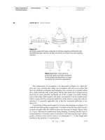
Figure 2.3: The element with the greatest gradient interpolation errors in Mesh 3.
Function values are indicated at the vertices and the interpolated function value is
shown.
is shown in Table 2.1. The largest interpolation error for mesh 1 is 1.3%, mesh 2 per-
forms slightly worse at 3.77% whereas the error for mesh 3 is almost 40%. The gradient
interpolation errors tell a similar story. Mesh 1 approximates the gradient within 5%
of the analytical value and mesh 2 is within 7% of the analytical value. However, the
greatest gradient interpolation error on mesh 3 is over 600%, rendering the approxi-
mation of this function and its gradient worthless. This simple example demonstrates
just how great an effect large angles can have on the accuracy of interpolated functions
and on their gradients. In many problems, for example, deformation of materials, the
gradient of the primary function (i.e. strain) is more important than the function itself.
Therefore the accuracy of the interpolated gradients are also of primary interest.
The source of these errors can be investigated by examining the element of Mesh 3
which gave the greatest gradient interpolation errors, Figure 2.3. The value of the
function is shown at each node and the value shown at the midpoint of the bottom
edge is the interpolated value,
0.255+0.005
2
. This interpolated value is independent of the
value of the top node. As the angle at the top node approaches 180
◦
, it becomes closer
and closer to the interpolated point. Therefore the vertical component of ∇g rapidly
becomes very large making it a very poor approximation of ∇f even though f = g at
each node.

Consider now the numerical integration of the function f over the domain. The effect of
2.1. Errors induced by poor meshes 7
Mesh 1 Mesh 2 Mesh 3
% error -2.0 -5.5 -20.874
Table 2.2: Numerical integration errors for each mesh
extreme internal angles is now demonstrated. A three point integration rule is adopted
which is sufficient to accurately integrate the function that is approximated using
linear interpolation functions. Thus any errors will be the result of an interpolation
error rather than insufficient integration points.
The larger an angle, the longer the edge opposite it, thus the larger the interpolation
error. It is trivial to analytically integrate the chosen function to get an exact answer.
Table 2.2 compares exact integration of the function with the numerical result. The
solutions for both Meshes 1 and 2 are reasonably accurate whereas the solution obtained
for Mesh 3 is very inaccurate. In the context of the Finite Element method, this
simple experiment clearly shows the need for high quality meshes as the quality of
the solution deteriorates rapidly as the quality of the mesh deteriorates. It is worth
noting that, in this very simple case, the use of quadratic elements instead of linear
elements would have yielded the correct solution. However in practice the function
being approximated can be orders of magnitude greater than the interpolation function
or not a polynomial.
These simple numerical experiments clearly demonstrate how the presence of large
angles in meshes can lead to errors in the FE solution.
2.1.2 The approximation of functions on anisotropic meshes
Many physical problems which are analysed using FEA involve functions whose so-
lutions vary significantly more in one direction than in the others [4]. Equilateral
elements are well suited to solution fields that vary equally in every direction however,
the use of isotropic elements in problems where the solution is highly anisotropic will
result in meshes which are prohibitedly large [5]. For example, problems involving
boundary layers and shock waves or flow problems with high Reynold’s number often
exhibit significant anisotropy. It may be advantageous to the accuracy and efficiency

of the numerical solution of such problems to use an anisotropic mesh. Furthermore,
the degree of anisotropy may vary over the entire mesh, meaning the definition of the
ideal element may be a function of the position of the element in the mesh. This is
2.1. Errors induced by poor meshes 8
Figure 2.4: (a) Plot of the function f(x, y) = x
2
. and (b) its discretisation using Mesh
3.
also true for functions which vary equally in each direction, as the magnitude of this
variation may change from point to point, meaning that although equilateral elements
may be suitable throughout the mesh, the size of the ideal element may vary according
to the position in the mesh.
In the previous section, the interpolation errors for three different meshes used to
approximate a function, f(x, y) = x
2
+
y
2
2
, were quantified. The curvature of this
function is both a function of position and direction. It was concluded in the previous
section that large angles lead to interpolation errors, and thus errors in the FE solution.
This is because the edge opposite a large angle is much longer than the other two edges
of the element. However, if the function being approximated is constant or varies
linearly over this edge, the presence of the large angle does not introduce errors.
This concept may be demonstrated by examining the function f (x, y) = x
2
, Figure 2.4.
This function is constant in the y direction, therefore the approximation of this function
using Mesh 3 is in fact quite accurate, despite Mesh 3 between completely unsuitable

in the previous example. This means that the choice of mesh is heavily influenced
by the function it must approximate. If the curvature of the function is isotropic,
then isotropic elements should be used. For functions whose curvature is anisotropic,
anisotropic elements, when correctly orientated, may be the most suitable. This is
because elements can be stretched to adapt to features which are of equal or lower
dimensionality than the element shape functions [6]. This then leads to the concept
of curvature adaptive meshing where the size, shape and orientation of elements is
chosen so as to account for the curvature of the function being approximated on the
mesh.
2.1.2.1 Curvature adaptive meshing
In the previous section it was shown that the suitability of a mesh for interpolating
a function is intrinsically linked to the curvature of the function that the mesh is ap-
2.1. Errors induced by poor meshes 9
proximating. This means that the mesh generation and optimisation processes should,
where possible, take this into account. The curvature of the underlying function may be
accounted for by defining a metric field, which is discussed in detail in the Section 2.1.3,
based on a computed solution on an existing mesh of a domain [7]. This is then used
as an input to a suitable mesh generation or optimisation package [5]. For example, in
a steady-state problem, where the solution does not change with time, a solution may
be obtained using an isotropic mesh. Using this solution, a metric field is then defined
and used to either re-mesh all or part of the domain or to optimise the mesh. The
problem is then solved again using the new mesh. This process may be repeated until
a satisfactory solution is obtained. Such a technique is suitable for problems where the
computational cost is relatively low thus allowing for multiple iterations of the solution
process on continuously improving meshes. However, the computational cost of solving
many interesting problems is such that this technique would be too expensive.
Schoen [2] proposes an alternative technique where the problem is solved on a coarse
isotropic mesh to obtain a rough estimate of the solution. Using metrics derived from
this mesh, a finer anisotropic mesh may be generated and a much more accurate solution
obtained. However, important features of the solution may not be captured by the

coarse mesh [6], thus they would not be accounted for by this process. This method
may be quite effective for repetitive steady-state calculations but it is not at all suitable
for transient problems [6] where the solution changes with time, such as the problem
studied in Chapter 7. This is both for cost and accuracy reasons. In such a problem,
the solution is calculated at intervals, or time-steps, using the solution at the previous
time-step. The solution at the start time is calculated using the initial conditions. A
metric field is calculated using the computed solution and the mesh is adapted. At
this stage, either the solution is re-calculated using the adapted mesh, or the solution
at the following time-step is calculated. In either case, a solution must be transferred
from an existing mesh to the new mesh. As shown in Section 2.1.1, the interpolation
of a solution from one mesh to another is a source of errors, thus, this would lead to an
inaccurate solution. At the starting time, the inital conditions may be applied to an
adapted mesh, such as in a steady-state problem, without any errors. This is because
the intial conditions are generally defined on the undiscretised domain, and not on
the discretised domain as is the case at intermediate time-steps. This is also true for
some steady-state problems where the load may be applied in stages so that the entire
solution path may be traced and to limit the accumulation of solution errors [8]. In
the following sections, the process of calculating a metric field is explained and several
possible methods proposed in the literature of adapting a mesh based on the metric
field are described.
2.1. Errors induced by poor meshes 10
2.1.3 The calculation of a metric field
A metric tensor is a function for calculating the distance between any two points in a
space [9]. Therefore, the explanation of a metric tensor requires the formal definition
of length [10]. The definition of length in a metric space requires both the metric used
to define the space and a suitable definition of the dot product. For any point P in R
d
,
a metric tensor is a d×d symmetric positive definite matrix M(P ). In two dimensions,
M(P ) takes the following form:

M(P ) =

a b
b c

(2.1)
where a > 0 and c > 0 and its determinant ac −b
2
> 0. This tensor must be symmetric
positive definite so that its geometric representation is an ellipse [5]. The coefficients
of the metric depend on the position P . This induces a Riemannian structure over R
d
.
If the coefficients of this matrix do not depend on P then the classical Euclidean case
is defined, where the metric is not a function of position [10].
Using equation 2.1, the dot product for a given metric M(P ) in Euclidean space for
two vectors u and v is defined as:
u, v
M(P )
= u
T
M(P )v (2.2)
Using the standard Euclidean norm, the norm of a vector is defined as:
u =

u, u
M(P )
=

u

T
M(P )u (2.3)
The calculation of the length of a vector is more complicated when the metric is a
function of the point P . For example, take a vector u connecting points a and b. To
calculate the length of this vector, the metrics at both a and b and each intermediate
metric must be considered [11]. This is achieved by using a parameterised segment,
γ(t) = a + tu. Therefore the length of a vector connecting two points, where the metric
is a function of position is defined in equation 2.4.
l
M
(u) =

1
0

u
T
M(t)u (2.4)
The is in contrast to the method presented by Thompson et al [7] where the length of
a vector is calculated using the average of the metric at both nodes.
2.1. Errors induced by poor meshes 11
2.1.4 Construction of a metric tensor using error indicators
The most common method of calculating metric tensors for use on finite element meshes
involves analysing error indicators. The simplest error indicator is obtained by evaluat-
ing the jump or absolute difference of the variable being interpolated along an edge [6].
A much more common method involves estimating the approximation error of the dis-
cretised function. Assuming the function is smooth, the error may be estimated to one
order greater than the order of the element shape functions [6]. The aim of this process
is to construct a metric which gives a homogeneous distribution of the interpolation
error over the entire mesh. This will be done in one dimension using a regular function

u which is defined on the segment [a, b]. Let h be the length of segment [a, b] which
is not necessarily small and Π
h
u be the P
1
interpolation of the function u on [a, b]
meaning that it is linear and piecewise continuous [12].
The following derivation is adapted from Frey and George [10]. As the interpolation
scheme is of P
1
type, the interpolation error is related to the variation of the various
variables being approximated on [a, b] and in particular, to their gradients and Hessians.
The function and its approximation are equal at a and b meaning that Π
h
u(a) = u(a)
and Π
h
u(b) = u(b). The approximation error is defined as e(x) = u(x) −Π
h
u(x).
Consider the function Π
h
u on the segment [Π
h
(a), Π
h
(b)]] which is the linear approx-
imation of the function u on the segment between a and b. It is assumed that the
computed solution is quite close to the actual solution. This analysis is based on a
variation of Taylor’s formula. Since h is not necessarily small, a formula of the type

shown in equation 2.5 is preferable to a standard Taylor series expansion [10].
f(x) = f (a) + (a −x)f

(x) +
(a −x)
2
2
f

(x + t(a − x)) (2.5)
where t, defined on the segment [0, 1], is a function of both x and a. For this analysis,
f is defined as (u −Π
h
u)(x) = u(x) −u
h
(x) on the segment [a, b]. Therefore the error
at point a is approximated using equation 2.6.
e(a) = (u−Π
h
u)(a) = (u−Π
h
u)(x)+(a−x)(u−Π
h
u)

(x)+
(a −x)
2
2
(u−Π

h
u)

(x+t
1
(a−x))
(2.6)
However, as previously stated, the function u and its approximation Π
h
u are equal
at a meaning that the left hand side is zero. This yields the following simplified
expression:
0 = (u −Π
h
u)(x) + (a − x)(u −Π
h
u)

(x) +
(a −x)
2
2
(u −Π
h
u)

(x + t
1
(a −x)) (2.7)
2.1. Errors induced by poor meshes 12

As the largest interpolation error is of interest here, the extremum x where (u −
Π
h
u)

(x) = 0 is sought. Therefore this expression may be further simplified.
0 = (u −Π
h
u)(x) +
(a −x)
2
2
(u −Π
h
u)

(x + t
1
(a −x)) (2.8)
A similar expression for b may also be constructed:
0 = (u −Π
h
u)(x) +
(b −x)
2
2
(u −Π
h
u)


(x + t
2
(b −x)) (2.9)
Adding equations 2.8 and 2.9 gives:
0 = 2(u−Π
h
u)(x)+
(a −x)
2
2
(u−Π
h
u)

(x+t
1
(a−x))+
(b −x)
2
2
(u−Π
h
u)

(x+t
2
(b−x))
(2.10)
Let M be the majorant of u


on the segment [a, b]. Therefore:
|(u −Π
h
u)(x)| ≤
1
2

(a −x)
2
2
+
(b −x)
2
2

M (2.11)
Then:
|(u −Π
h
u)(x)| ≤
1
4
max
x∈[a,b]

(a −x)
2
+ (b − x)
2


M (2.12)
The maximum is reached for
a+b
2
, implying that, ∀x ∈ [a, b]:
|e(x)| = |(u −Π
h
u)(x)| ≤
(b −a)
2
8
M (2.13)
The value of
(b−a)
2
8
M is compared with a given value , which is the maximum allowable
error or the maximum allowed gap between the function u and its linear approximation
Π
h
u. In many transient problems this error tolerance may be required to vary over the
domain [6]. The calculation of M via the recovery of the Hessian on the segment [a, b]
is described in the next section.
Hessian recovery
The next step in developing a metric tensor based on error analysis involves recovering
the Hessian of the function being approximated. The following derivation is adapted
from Löhner [6]. This method involves the assumption that the Hessian may be ex-
pressed using shape functions

N. Therefore:

∂
2
u
∂s
2
≈

Nu

(2.14)