on the angular momentum of light
Bạn đang xem bản rút gọn của tài liệu. Xem và tải ngay bản đầy đủ của tài liệu tại đây (9.09 MB, 144 trang )
Glasgow Theses Service
Cameron, Robert P. (2014) On the angular momentum of light.
PhD thesis.
Copyright and moral rights for this thesis are retained by the author
A copy can be downloaded for personal non-commercial research or
study, without prior permission or charge
This thesis cannot be reproduced or quoted extensively from without first
obtaining permission in writing from the Author
The content must not be changed in any way or sold commercially in any
format or medium without the formal permission of the Author
When referring to this work, full bibliographic details including the
author, title, awarding institution and date of the thesis must be given
On the Angular Momentum of Light
Robert P Cameron BSc (Hons)
Submitted in fulfillment of the requirements for the degree of Doctor of Philosophy
School of Physics and Astronomy
College of Science of Engineering
University of Glasgow
04/12/2014
Declaration
The research described in this thesis is my own, except where otherwise stated.
Robert P Cameron BSc (Hons)
i
Abstract
The idea is now well established that light possesses angular momentum and that this comes in
two distinct forms, namely spin and orbital angular momentum which are associated with circular
polarisation and helical phase fronts respectively. In this thesis, we explain that this is, in fact, a mere
glimpse of a much larger picture: light possesses an infinite number of distinct angular momenta,
the conservation of which in the strict absence of charge reflects the myriad rotational symmetries
then inherent to Maxwell’s equations. We recognise, moreover, that many of these angular momenta
can be identified explicitly in light-matter interactions, which leads us in particular to identify new
possibilites for the use of light to probe and manipulate chiral molecules.
ii
Acknowledgements
This was the most difficult part of my thesis to write: whenever I think I’m done, I find that I’ve left
some people out!
Mum and dad; it was your idea to send me to university. I hope I didn’t let you down. Thank you for
supporting my efforts to better understand the how and the why of things. Steve and Alison; thank
you for taking me on (and keeping me) as a PhD student. I don’t know where I’d be now were it not for
your guidance and patience over the last three years. Fiona; I should have listened to you when you
told me to use BibTex (and perhaps in general). Thank you for helping me to rectify my mistake(s).
And for listening to my thesis. To the many, many other people who I’ve not yet mentioned explicitly
(Gergeley, Thomas, Sarah, Václav, Graeme, Matthias, Andrew, Sonja, Mohamed, Drew, Amaury,
Corey, Cameron, Jamie, Paul, Ziggy, ), I am, of course, very grateful.
The research described in this thesis was supported by The Carnegie Trust for the Universities of
Scotland.
iii
Publications
1. R. P. Cameron, S. M. Barnett and A. M. Yao. Optical helicity, optical spin and related quantities
in electromagnetic theory. New Journal of Physics, 14:053050, 2012.
2. S. M. Barnett, R. P. Cameron and A. M. Yao. Duplex symmetry and its relation to the conser-
vation of optical helicity. Physical Review A 86:013845, 2012.
3. R. P. Cameron and S. M. Barnett. Electric-magnetic symmetry and Noether’s theorem. New
Journal of Physics 14:123019, 2012.
4. R. P. Cameron. On the ‘second potential’ in electrodynamics. Journal of Optics 16:015708,
2013.
5. R. P. Cameron, S. M. Barnett and A. M. Yao. Discriminatory optical force for chiral molecules.
New Journal of Physics 16:013020, 2014.
6. R. P. Cameron, S. M. Barnett and A. M. Yao. Optical helicity of interfering waves. Journal of
Modern Optics 61:25-31, 2014.
7. R. P. Cameron, A. M. Yao and S. M. Barnett. Diffraction gratings for chiral molecules and their
applications. Journal of Physical Chemistry A 118:3472-3478, 2014.
8. R. P. Cameron and S. M. Barnett. Optical activity in the scattering of structured light. Physical
Chemistry Chemical Physics 16:25819-25829, 2014.
9. R. P. Cameron, F. C. Speirits, C. R. Gilson, L. Allen and S. M. Barnett. The azimuthal compo-
nent of Poynting’s vector and the angular momentum of light. To be submitted, 2014.
iv
Summary
The original research described in this thesis spans a collection of topics in the theory of electrody-
namics, each of which touches upon the angular momentum of light. Our interest lies primarily in the
classical domain, although on occasion we delve into the quantum and semiclassical domains. The
structure and content of the thesis may be summarised as follows.
In §1, we review certain well established results in the theory of electrodynamics. These have been
chosen so as to make the thesis essentially self contained and should therefore be sufficient to un-
derstand the discussions that follow in §2-§5.
In §2, we make some rather formal observations about the theory of electrodynamics that under-
pin much of what follows in §3-§5. We begin by considering Maxwell’s equations as written in the
strict absence of charge and recall that these place the electric field E and the magnetic flux density
B on equal footing, which permits the introduction, in addition to the familiar ‘first potential’ A
⊥
, of
a ‘second potential’ C
⊥
. This leads us to observe in turn that the equations exhibit a remarkable
self-similarity as one considers various integrals (such as A
⊥
and C
⊥
) of E and B, as well as var-
ious derivatives of E and B. Finally, we allow for the presence of electric charge and generalise
some of our observations. In particular, we introduce and examine a seemingly reasonable general
definition of C
⊥
; a non-trivial problem, owing to the breakdown of electric-magnetic discrimination
that accompanies the charge.
In §3, we turn our attention to the angular momentum of light and its fundamental description in
the theory of electrodynamics. Again, we begin by considering light that is propagating freely in
the strict absence of charge. The fact is well established that such light possesses rotation angular
momentum
J =
∞
r ×(E × B) d
3
r
and boost angular momentum
K =
∞
t E × B −
1
2
r (E · E + B · B)
d
3
r
and that the conservation of the rotation angular momentum J is associated with circular rotations in
space whereas the conservation of the boost angular momentum K is associated with boosts, which
can be regarded as hyperbolic rotations in spacetime. It is known, moreover, that the rotation angular
momentum J can itself be separated into independently conserved parts S and L that resemble
what we might expect of spin and orbital angular momentum
1
. It has been shown, however, that the
operators
ˆ
S and
ˆ
L representing the spin S and orbital angular momentum L do not obey the usual
angular momentum commutation relations, which has cast doubt upon their physical signifiance, al-
though each is, nevertheless, associated with a rotational symmetry.
1
An analogous separation for the boost angular momentum K yields a vanishing boost spin candidate and a non-
vanishing boost orbital angular momentum candidate which thus comprises the totality of the boost angular momentum.
v
This controversial result, taken together with a simple idea familiar from particle physics, leads us
to discover that light in fact possesses an infinite number of distinct angular momenta, which we
recognise as being such because they have the dimensions of an angular momentum and are con-
served. Spin and orbital angular momentum are but two of these. We attempt to elucidate the
physical significance of the angular momenta and their conservation, as well as the similarities, rela-
tionships and distinctions between them, through various analogies and explicit examples. Moreover,
we disambiguate the angular momenta from related but distinct properties of light such as the zilch
Z
αβ
, the conservation of which we interpret as being a reflection of the self-similarity that we un-
earthed in §2. Finally, we allow for the presence of charge and generalise some of our observations,
finding in particular that the definition of C
⊥
in the presence of charge that we proposed in §2 is
indeed a reasonable one.
In §4, we introduce a variational description of freely propagating light that places E and B on equal
footing, much in the spirit of §2. We use this description, together with Noether’s theorem, to study
symmetries and the conservation laws with which they are associated. This yields, in particular, a
more fundamental perspective on the angular momenta discovered in §3: the conservation of the
angular momenta, which are infinite in number, reflects the existence of an infinite number of ways in
which it is possible to rotate freely propagating light. Additional heirarchies of symmetries and asso-
ciated conservation laws, amongst them the conservation of Z
αβ
, are also identified and attributed
again to the self-similarity that we unearthed in §2.
In §5, we identify applications centred upon some of the angular momenta discovered in §3. Specif-
ically, we observe that many optical activity phenomena: light-matter interactions in which left-
and right-handed circular polarisations are distinguished, can be related explicitly to helicity, spin,
etc. This is unsurprising, perhaps, given that these angular momenta differ in value for left- and
right-handed circularly polarised light. We employ this new insight in the consideration of a well-
established manifestation of optical activity (optical rotation), a dormant manifestation of optical ac-
tivity (differential scattering) and a new manifestation of optical activity (discriminatory optical force
for chiral molecules). The latter two may be developed into powerful new techniques for the probing
and manipulation of chiral molecules.
We conclude in §6 by outlining possibilities for future research into chirality and optical activity which
follow on from the research presented in §5.
vi
Contents
1 Supporting Theory 1
1.1 Introduction . . . . . . . . . . . . . . . . . . . . . . . . . . . . . . . . . . . . . . . . 1
1.2 Classical electrodynamics . . . . . . . . . . . . . . . . . . . . . . . . . . . . . . . . 1
1.3 Quantum electrodynamics . . . . . . . . . . . . . . . . . . . . . . . . . . . . . . . . 13
1.4 The semiclassical approximation and induced multipole moments . . . . . . . . . . . 20
1.5 Angular momentum: some terminology . . . . . . . . . . . . . . . . . . . . . . . . . 23
2 Electric-Magnetic Democracy, the ‘Second Potential’ and the Structure of Maxwell’s
Equations 25
2.1 Introduction . . . . . . . . . . . . . . . . . . . . . . . . . . . . . . . . . . . . . . . . 25
2.2 In the strict absence of charge . . . . . . . . . . . . . . . . . . . . . . . . . . . . . . 25
2.3 In the presence of charge . . . . . . . . . . . . . . . . . . . . . . . . . . . . . . . . . 28
2.4 Discussion . . . . . . . . . . . . . . . . . . . . . . . . . . . . . . . . . . . . . . . . . 30
3 The Angular Momentum of Light 31
3.1 Introduction . . . . . . . . . . . . . . . . . . . . . . . . . . . . . . . . . . . . . . . . 31
3.2 Review of previously established results . . . . . . . . . . . . . . . . . . . . . . . . . 32
3.3 Intrinsic rotation angular momenta . . . . . . . . . . . . . . . . . . . . . . . . . . . . 36
3.4 The zilch . . . . . . . . . . . . . . . . . . . . . . . . . . . . . . . . . . . . . . . . . . 50
3.5 Extrinsic and quasi-extrinsic rotation angular momenta . . . . . . . . . . . . . . . . . 52
3.6 Boost angular momenta . . . . . . . . . . . . . . . . . . . . . . . . . . . . . . . . . . 53
3.7 In the presence of charge . . . . . . . . . . . . . . . . . . . . . . . . . . . . . . . . . 56
3.8 Discussion . . . . . . . . . . . . . . . . . . . . . . . . . . . . . . . . . . . . . . . . . 59
4 Noether’s Theorem and Electric-Magnetic Democracy 61
4.1 Introduction . . . . . . . . . . . . . . . . . . . . . . . . . . . . . . . . . . . . . . . . 61
4.2 Formalism . . . . . . . . . . . . . . . . . . . . . . . . . . . . . . . . . . . . . . . . . 61
4.3 Local symmetry transformations and their associated conservation laws . . . . . . . 68
4.4 Non-local symmetry transformations and their associated conservation laws . . . . . 75
4.5 Discussion . . . . . . . . . . . . . . . . . . . . . . . . . . . . . . . . . . . . . . . . . 82
5 Chirality and Optical Activity 84
5.1 Introduction . . . . . . . . . . . . . . . . . . . . . . . . . . . . . . . . . . . . . . . . 84
5.2 Optical rotation . . . . . . . . . . . . . . . . . . . . . . . . . . . . . . . . . . . . . . 86
vii
5.3 Differential scattering . . . . . . . . . . . . . . . . . . . . . . . . . . . . . . . . . . . 93
5.4 Discriminatory optical force for chiral molecules . . . . . . . . . . . . . . . . . . . . . 105
5.5 Discussion . . . . . . . . . . . . . . . . . . . . . . . . . . . . . . . . . . . . . . . . . 117
6 Future Research 118
viii
Chapter 1
Supporting Theory
1.1 Introduction
Electrodynamics; a word coined by Ampère [1], is concerned with (electrically)
1
charged matter,
the electromagnetic field and their mutual interaction. It is understood, at present, that the elec-
tromagnetic interaction is responsible for all phenomena not attributable instead to the gravitational
interaction, the strong interaction or the weak interaction
2
[8]; from the structure and properties of
molecules and atoms which comprise the material world around us to the light radiated by the stars
in the night sky [2, 3, 9–14].
The original research described in this thesis spans a collection of topics in the theory of electro-
dynamics, each of which touches upon the angular momentum of light. We begin in the present
chapter by summarising the well established results that support the discussions in §2-§5.
Throughout, we imagine ourselves to be in an inertial frame of reference with time t and a right-
handed Cartesian coordinate system: x, y and z, unless otherwise stated. Complex quantities are
indicated as such using a tilde, with complex conjugation indicated using an asterisk. Quantum oper-
ators are indicated as such using a circumflex, with Hermitian conjugation indicated using a dagger.
Unit vectors are indicated as such using a double circumflex. In the present chapter, as well as §2-§4,
we adopt a modified version of the international system of units in which the electric constant
0
, the
magnetic constant µ
0
and hence the speed of light in vacuum c = 1/
√
0
µ
0
are equal to unity. In
§1.4 and §5, we revert, however, to the international system of units as it is usually recognised.
1.2 Classical electrodynamics
In §2-§5, we work within the classical domain, unless otherwise stated. In the present section,
we therefore summarise some well established results from the theory of classical electrodynamics
[2, 3, 9–11, 14].
1
Magnetically charged matter is occasionally considered in theory [2–7], although, at the time of writing, it has not
been observed in experiment.
2
The electromagnetic and weak interactions themselves comprise a unified electroweak interaction [8]. In this thesis,
we neglect the influence of the weak interaction.
1
1.2.1 The microscopic equations
Consider N point particles of charge q
n
, mass
3
m
n
and position r
n
= r
n
(t) (n = 1, . . . , N ) which
give rise to a microscopic charge density ρ = ρ (r, t) and a microscopic current density J = J (r, t)
as
ρ =
N
n=1
q
n
δ
3
(r −r
n
) , (1.1)
J =
N
n=1
q
n
˙
r
n
δ
3
(r −r
n
) , (1.2)
with r = x
ˆ
ˆ
x + y
ˆ
ˆ
y + z
ˆ
ˆ
z the position vector with
ˆ
ˆ
x,
ˆ
ˆ
y and
ˆ
ˆ
z unit vectors in the +x, +y and +z
directions, δ
3
(r) a three-dimensional Dirac delta function and an overdot, notation due to Newton
[15], indicating a derivative with respect to time t. The trajectory of the nth particle is governed by
the Newton-Einstein-Lorentz equation [16, 17]:
d
dt
m
n
˙
r
n
1 −|
˙
r
n
|
2
= q
n
[E (r
n
, t) +
˙
r
n
× B (r
n
, t)] , (1.3)
whilst the microscopic electric field E = E (r, t) and the microscopic magnetic flux density B =
B (r, t) are governed by Maxwell’s equations [17, 18]:
∇ ·E = ρ, (1.4)
∇ ·B = 0, (1.5)
∇ ×E = −
˙
B, (1.6)
∇ ×B = J +
˙
E, (1.7)
with ∇ the gradient operator with respect to r. (1.4) is Gauss’s law, (1.5) is the analogue of Gauss’s
law for magnetism, (1.6) is the Faraday-Lenz law and (1.7) is Ampère’s law as corrected by Maxwell
[18], all in differential form, of course [2, 3, 9–11].
These equations (1.1)-(1.7) constitute an essentially complete statement of the theory of classical
electrodynamics. Solving them requires finding the r
n
, E and B.
1.2.2 Scalar and magnetic vector potentials
Gauss’s law for magnetism (1.5) and the Faraday-Lenz law (1.6) do not depend explicitly upon the
particles and may be viewed, therefore, as geometrical identities obeyed by E and B. They can be
solved by taking
E = −∇Φ −
˙
A, (1.8)
B = ∇ ×A, (1.9)
3
More precisely, m
n
is the bare rest mass of the nth particle [11].
2
for any scalar potential
4
Φ = Φ (r, t) and magnetic vector potential A = A (r, t). To be consistent
with the Newton-Einstein-Lorentz equation (1.3), Gauss’s law (1.4) and the Ampère-Mawell law (1.7),
we then require that
d
dt
m
n
˙
r
n
1 −|
˙
r
n
|
2
= q
n
−∇Φ (r
n
, t) −
˙
A (r
n
, t) +
˙
r
n
× [∇ × A (r
n
, t)]
, (1.10)
−∇
2
Φ −∇ ·
˙
A = ρ, (1.11)
−∇
2
A + ∇ (∇ ·A) = J −∇
˙
Φ −
¨
A, (1.12)
with ∇
2
= ∇ ·∇ the Laplacian operator with respect to r. In moving our focus from the six quantities
that are the components of E and B to the four quantities that are Φ and the components of A, we
must pay the price of going from three equations (1.3) that are zeroth order in temporal and spatial
derivatives and eight equations (1.4)-(1.7) that are first order, to three equations (1.10) that are in-
stead first order and four equations (1.11)-(1.12) that are instead second order.
Φ and A are not uniquely defined in that E and B are unchanged by the transformation [19]
Φ → Φ + ˙χ
A → A −∇χ, (1.13)
for any time-odd Lorentz scalar field χ = χ (r, t); a so-called gauge function [2, 3, 9–11]. This
freedom permits us to ‘choose a gauge’, by imposing a condition upon ∇ ·A. The Coulomb gauge
5
:
∇ ·A = 0, (1.14)
and a Lorenz gauge
6
[20]:
∇ ·A +
˙
Φ = 0, (1.15)
are but two examples of gauge choices.
1.2.3 Special relativity
In the theory of special relativity [2, 3, 10, 16, 21], the time t = x
0
and spatial coordinates x = x
1
,
y = x
2
and z = x
3
with which we have chosen to describe events are recognised as being the
components of the position four vector x
α
= (t, r). Raised indices taken from the start of the Greek
alphabet (α, β, . . . ), including α here, are referred to as being contravariant and can take on the
values 0, corresponding to time, and 1, 2 and 3, corresponding to space. Letters taken from the start
of the Roman alphabet (a, b, . . . ), when employed as contravariant indices, may assume the values
1, 2 and 3 corresponding to space only.
4
From here onwards, it is to be understood where relevant that quantities are ‘microscopic’, unless otherwise stated.
5
The Coulomb gauge condition can be seen in Maxwell’s original work [18].
6
There are, in fact, many Lorenz gauges, for a so-called restricted gauge transformation, with ∇
2
χ − ¨χ = 0, maintains
the equality seen in (1.15) [2].
3
The principle of special relativity, due to Einstein [16], tells us in particular that the laws of physics,
whilst holding in the x
α
coordinate system, should also hold in all other coordinate systems x
α
=
(t
, r
) related to x
α
as
x
α
= Λ
α
α
x
α
, (1.16)
with the array of constants Λ
α
α
describing (proper) rotations and / or boosts and where we have
introduced the summation convention, also due to Einstein [22]: here and in what follows, it is to be
understood that a double appearance of an index implies summation over its allowed values. For x
α
rotated relative to x
α
about the +z axis through an angle θ in the usual sense, given by the right-hand
rule;
Λ
α
α
=
1 0 0 0
0 cos θ sin θ 0
0 −sin θ cos θ 0
0 0 0 1
, (1.17)
whereas for a boost in standard configuration of x
α
relative to x
α
in the +z direction with speed v
and associated rapidity φ = arctan v;
Λ
α
α
=
cosh φ −sinh φ 0 0
−sinh φ cosh φ 0 0
0 0 1 0
0 0 0 1
, (1.18)
to give but two explicit examples [2, 3, 10, 14, 21]. Reciprocally,
x
α
= Λ
α
α
x
α
(1.19)
with the array Λ
α
α
being the inverse of Λ
α
α
, of course. More generally, an object with components
described by r (r = 0, 1, . . . ) raised indices, the values X
α
β
ω
of which in x
α
are related to those
X
αβ ω
in x
α
as
X
α
β
ω
= Λ
α
α
Λ
β
β
. . . Λ
ω
ω
X
αβ ω
, (1.20)
is said to be a contravariant tensor of rank r.
The partial derivatives ∂
t
= ∂
0
, ∂
x
= ∂
1
, ∂
y
= ∂
2
and ∂
z
= ∂
3
are recognised as being the compo-
nents of the partial derivative four vector ∂
α
= (∂
t
, ∇). Lowered indices taken from the start of the
Greek alphabet, including α here, are referred to as being covariant and, like contravariant indices,
can also take on the values 0, corresponding to time, and 1, 2 and 3, corresponding to space. Let-
ters taken from the start of the Roman alphabet, when employed as covariant indices, may assume
the values 1, 2 and 3 corresponding to space only. The components ∂
α
= (∂
t
, ∇
) of the partial
derivative four vector in x
α
= (t
, r
) are related to those ∂
α
in x
α
as
∂
α
= Λ
α
α
∂
α
. (1.21)
4
More generally, an object with components described by r (r = 0, 1, . . . ) lowered indices, the values
X
α
β
ω
of which in x
α
are related to those X
αβ ω
in x
α
as
X
α
β
ω
= Λ
α
α
Λ
β
β
. . . Λ
ω
ω
X
αβ ω
, (1.22)
is said to be a covariant tensor of rank r.
We now introduce the Minkowski metric tensor η
αβ
= η
αβ
= diag (1, −1, −1, −1) which plays a
dual role in that it defines the spacetime interval dτ between events at x
α
and x
α
+ dx
α
as
dτ
2
= η
αβ
dx
α
dx
β
(1.23)
and can be used to interconvert contravariant and covariant indices as
η
αβ
X
β
= X
α
, (1.24)
X
α
= η
αβ
X
β
, (1.25)
for example [2, 21]. Thus, we can have so-called mixed tensors, which possess both contravariant
and covariant indices, an example of which is the Kronecker delta tensor δ
α
β
= diag (1, 1, 1, 1). Fi-
nally, let us introduce the Levi-Civita pseudotensor
7
αβγδ
, defined as
0123
= 1 whilst alternating in
sign under exchange of any two of these indices and having the remainder of its components vanish
[2, 10, 21].
The significance of this formalism lies in the fact that an equation that holds in x
α
and is express-
ible in terms of tensors and pseudotensors manifestly holds with the same form in x
α
[21]. This is
true in particular of the results presented in §1.2.1 and §1.2.2. To demonstrate this, let us introduce
the position four vector x
α
n
= (t, r
n
) of the nth particle, the linear-momentum moment four vector
p
α
n
= m
n
(1,
˙
r
n
) /
1 −|
˙
r
n
|
2
of the nth particle, the current four vector J
α
= (ρ, J) and a magnetic
potential four vector A
α
= (Φ, A). The electromagnetic field tensor F
αβ
and the dual electromag-
netic field pseudotensor G
αβ
are defined in turn as
F
αβ
= ∂
α
A
β
− ∂
β
A
α
, (1.26)
G
αβ
=
αβγδ
F
γδ
/2. (1.27)
In matrix form
F
αβ
=
0 −E
x
−E
y
−E
z
E
x
0 −B
z
B
y
E
y
B
z
0 −B
x
E
z
−B
y
B
x
0
(1.28)
7
As we have restricted our attention here to the proper (and homogeneous) transformations (1.20) and (1.22), the
distinction between tensors and pseudotensors is of no consequence. The distinction is important, however, if we allow for
improper transformations, specifically with inversions of spatial coordinates [2, 10].
5
and
G
αβ
=
0 −B
x
−B
y
−B
z
B
x
0 E
z
−E
y
B
y
−E
z
0 E
x
B
z
E
y
−E
x
0
. (1.29)
We have then that
dp
α
n
/dτ
n
= q
n
F
βα
(x
n
) dx
nβ
/dτ
n
, (1.30)
∂
β
F
αβ
= −J
α
, (1.31)
∂
β
G
αβ
= 0, (1.32)
with dτ
n
=
1 −|
˙
r
n
|
2
dt a proper time interval for the nth particle. For α = 0, (1.30) describes
the rate of change of energy of the nth particle and for α = 1, 2 and 3 yields the x, y and z com-
ponents of the Newon-Einstein-Lorentz force law (1.3). For α = 0, (1.31) is Gauss’s law (1.4) and
for α = 1, 2 and 3 yields the x, y and z components of the Ampère-Maxwell law (1.7). For α = 0,
(1.32) is Gauss’s law for magnetism (1.5) and for α = 1, 2, 3 yields the x, y, z components of the
Faraday-Lenz law (1.6). Thus, the classical theory of electrodynamics manifestly respects the princi-
ple of special relativity, as claimed [2, 3, 10, 14, 21].
On occasion, we will find it useful to consider x
α
together with coordinate systems x
α
related to
x
α
as above but with boosts excluded. Quantities that transform analogously to r in this restricted
three-dimensional sense are referred to as being rotational tensors and rotational pseudotenors [2].
Vectors and pseudovectors are thus rotational tensors and rotational pseudotensors of rank one.
We label the components of rotational tensors and pseudotensors using indices taken from the start
of the Roman alphabet in parenthesis. These may assume the values 1, 2 and 3 corresponding to
space only and we make no dinstinction between raised and lowered forms, taking
A
1
= −A
1
= A
(1)
= A
(1)
= A
x
, (1.33)
A
a
A
a
= −A
(a)
A
(a)
= −A
(a)
A
(a)
= −A
(a)
A
(a)
= −A
2
x
− A
2
y
− A
2
z
, (1.34)
for example. Of particular use to us is the Kronecker delta rotational tensor δ
(ab)
= diag (1, 1, 1) and
the Levi-Civita rotational pseudotensor
(abc)
, defined as
(123)
= 1 whilst alternating in sign under
exchange of any two of these indices and having the remainder of its components vanish.
1.2.4 Conservation laws
It is required by Gauss’s law (1.4) and the Ampère-Maxwell law (1.7) and indeed follows from the
definitions seen in (1.1) and (1.2) that
˙ρ + ∇ ·J = 0. (1.35)
6
The significance of (1.35) may be seen by integrating both sides over a finite volume V with bounding
surface S and making use of Gauss’s integral theorem [3], thus obtaining
d
dt
V
ρ d
3
r = −
S
J ·d
2
r, (1.36)
which tells us that changes in t of the charge
V
ρ d
3
r contained in V are compensated for by
an equal and opposite flux
S
J · d
2
r of charge through S. Hence, (1.35) is said to be a continuity
equation for charge and its integral solution (1.36) is said to be a local conservation law for charge.
If V now extends over all space, (1.36) becomes
d
dt
∞
ρ d
3
r =
dQ
dt
= 0, (1.37)
with Q =
N
n=1
q
n
the total charge of the particles. This (1.37) is said to be a global conservation
law for charge.
Such mathematical arguments are independent of the physical nature of charge and it is clear, there-
fore, that any equation of the form seen in (1.35) embodies the local and hence global conservation
of a quantity. It will be noticed that (1.35) is ∂
α
J
α
= 0. We should be clear, however, that the principle
of special relativity does not require a continuity equation to be expressible in terms of tensors and /
or pseudotensors, in general.
1.2.5 Solenoidal and irrotational pieces, reciprocal space and the normal variables
The observation is attributed to Helmholtz [23] that a vector field or pseudovector field V = V (r, t)
can be separated into a solenoidal piece V
⊥
and an irrotational piece V
as
V = V
⊥
+ V
, (1.38)
with ∇ · V
⊥
= 0 and ∇ ×V
= 0, by definition [2, 3, 11, 12]. The significance of such separations
is clearer, perhaps, in reciprocal rather than ordinary space. To illustrate this, let us introduce in a
general manner the spatial Fourier transform
˜
Y =
˜
Y (k, t) of a real field Y = Y (r, t) in ordinary
space as [11]
˜
Y =
∞
1
2
√
2π
3
Y exp (−ik ·r) d
3
r, (1.39)
with k a wavevector. It is then found that the spatial Fourier transforms
˜
V
⊥
and
˜
V
of V
⊥
and
V
satisfy k ·
˜
V
⊥
= 0 and k ×
˜
V
= 0 and are thus everywhere perpendicular and parallel to k
in reciprocal space. For this reason,
˜
V
⊥
and
˜
V
are sometimes referred to as the transverse and
7
Figure 1.1: The spatial Fourier transform
˜
V (k, t) of a vector or pseudovector field V (r, t) can be separated
into a transverse piece
˜
V
⊥
(k, t) and a longitudinal piece
˜
V
(k, t), which are everywhere perpendicular and
parallel to k in reciprocal space, as depicted here. We have taken
˜
V (k, t) to be real for the sake of illustration.
longitudinal pieces of the spatial Fourier transform
˜
V of V [11, 12]: see figure 1.1. Thus,
˜
V
⊥
(a)
=
ˆ
ˆ
k
(a)
ˆ
ˆ
k
(b)
˜
V
(b)
, (1.40)
˜
V
(a)
=
δ
(ab)
−
ˆ
ˆ
k
(a)
ˆ
ˆ
k
(b)
˜
V
(b)
, (1.41)
from which it follows that
V
⊥
(a)
=
∞
δ
⊥
(ab)
r −r
V
(b)
r
d
3
r
, (1.42)
V
(a)
=
∞
δ
(ab)
r −r
V
(b)
r
d
3
r
, (1.43)
with δ
⊥
(ab)
(r) the so-called transverse delta function and δ
(ab)
(r) the so-called longitudinal delta func-
tion, given by [11, 12]
δ
⊥
(ab)
(r) =
2
3
δ
(ab)
δ
3
(r) −
1
4π|r|
3
δ
(ab)
−
ˆ
ˆr
(a)
ˆ
ˆr
(b)
, (1.44)
δ
(ab)
(r) =
1
3
δ
(ab)
δ
3
(r) +
1
4π|r|
3
δ
(ab)
−
ˆ
ˆr
(a)
ˆ
ˆr
(b)
. (1.45)
Such separations are not obviously expressible using the language of tensors and pseudotensors in-
herent to the theory of special relativity and there exists no simple relationship between V
⊥
and V
and their counterparts in another coordinate system x
α
, in general [11]. They nevertheless appear
naturally in many contexts and yield important insights. Amongst these lies the fact that a gauge
transformation (1.13) changes Φ and the irrotational piece A
of A whilst leaving the solenoidal
piece A
⊥
of A unchanged. Thus, it is Φ and A
in particular that suffer the gauge freedom of the
electromagnetic field whereas A
⊥
is, in fact, uniquely defined [11].
Of particular interest to us are the normal variables
˜
α =
˜
α (k, t) in reciprocal space which are
8
transverse (k ·
˜
α = 0) and governed by the equations
8
˙
˜
α + i|k|
˜
α =
i
2|k|
˜
J
⊥
. (1.46)
The
˜
α evolve independently of each other in t when the spatial Fourier transform
˜
J
⊥
of the solenoidal
piece J
⊥
of J vanishes (
˜
J
⊥
= 0). Their introduction can be traced back at least as far as the work of
Darwin [24]. The solenoidal piece E
⊥
of E, B and A
⊥
are determined by the
˜
α as [11]
E
⊥
=
∞
i
4
|k|
π
3
[
˜
α exp (ik · r) −
˜
α
∗
exp (−ik · r)] d
3
k, (1.47)
B =
∞
i
4
π
3
|k|
k ×[
˜
α exp (ik · r) −
˜
α
∗
exp (−ik · r)] d
3
k, (1.48)
A
⊥
=
∞
1
4
π
3
|k|
[
˜
α exp (ik · r) +
˜
α
∗
exp (−ik · r)] d
3
k. (1.49)
In contrast, the irrotational piece E
of E is determined by the r
n
as [11]
E
=
∞
ρ (r
, t) (r − r
)
4π|r −r
|
3
d
3
r
=
N
n=1
q
n
(r −r
n
)
4π|r − r
n
|
3
, (1.50)
this being the non-retarded
9
Coulomb field of the particles. Thus, the dynamical degrees of freedom
of the electromagnetic field are embodied by the
˜
α and are exhibited by E
⊥
and B, which we refer to
collectively as the radiation field [11–13]. Of course, (1.46) must be solved simultaneously with the
Newton-Einstein-Lorentz equation (1.3), in general. Knowledge of the
˜
α together with the r
n
then
constitutes an essentially complete description of the system, one with minimal redundancy [11].
1.2.6 Partitioning ρ and J and the transition to the macroscopic domain
It is often convenient to partition ρ and J into pieces of distinct character. For a single molecule or
atom, with some of the N particles being electrons whilst the remainder are nuclei, we take [11, 12]
ρ = ρ
f
− ∇ · P, (1.51)
J = J
f
+
˙
P + ∇ × M + J
R
, (1.52)
8
The
˜
α here are larger than those defined in the book by Cohen-Tannoudji, Dupont-Roc and Grynberg [11], for
example, by a factor of
√
¯h, with ¯h the reduced Planck constant.
9
Like E
, E
⊥
also exhibits non-retarded behaviour such that E itself is retarded [11].
9
for
ρ
f
= Q δ
3
(r −R) , (1.53)
P =
N
n=1
q
n
(r
n
− R)
1
0
δ
3
[r −R − u (r − r
n
)] du, (1.54)
J
f
= Q
˙
R δ
3
(r −R) , (1.55)
M =
N
n=1
q
n
(r
n
− R) × (
˙
r
n
−
˙
R)
1
0
u δ
3
[r −R − u (r − r
n
)] du, (1.56)
J
R
= ∇ × (P ×
˙
R), (1.57)
with R = R (t) the position of a point in the vicinity of the particles that may coincide with the position
of their centre of energy but need not neccesarily. The free charge density ρ
f
describes a single point
charge Q located at R. The components P
(a)
of the polarisation P can be expanded as [11, 12]
P
(a)
=
∞
i=1
(−1)
i+1
d
(i)
(aa
2
a
i
)
∂
a
2
. . . ∂
a
i
δ
3
(r −R) , (1.58)
with the components d
(i)
(a
1
a
2
a
i
)
= d
(i)
(a
1
a
2
a
i
)
(t) of the ith (i = 1, 2 . . . ) electric multipole moment of
the molecule or atom’s charge distribution
10
defined here by us as being
d
(i)
(a
1
a
2
a
i
)
=
N
n=1
q
n
i!
(r
n
− R)
(a
1
)
(r
n
− R)
(a
2
)
. . . (r
n
− R)
(a
i
)
. (1.59)
The free current density J
f
describes a single point charge Q located at R moving with velocity
˙
R.
The magnetisation M can be expanded as [11, 12]
M
(a)
=
∞
i=1
(−1)
i+1
m
(i)
(aa
2
a
i
)
∂
a
2
. . . ∂
a
i
δ
3
(r −R) , (1.60)
with the components m
(i)
(a
1
a
2
a
i
)
= m
(i)
(a
1
a
2
a
i
)
(t) of the ith (i = 1, 2 . . . ) magnetic multipole moment
of the molecule or atom’s current distribution defined here by us as being
m
(i)
(a
1
a
2
a
i
)
=
N
n=1
q
n
i
(i + 1)!
(r
n
− R) × (
˙
r
n
−
˙
R)
(a
1
)
(r
n
− R)
(a
2
)
. . . (r
n
− R)
(a
i
)
. (1.61)
The Röntgen current density J
R
describes a relativistic effect: should the molecule or atom possess
a non-vanishing P and be translating with non-vanishing velocity
˙
R, it will possess an apparent mag-
netisation of P ×
˙
R [12]. ρ
f
and J
f
happen to vanish (ρ
f
= 0, J
f
= 0) of course, owing to the electric
neutrality (Q = 0) of the molecule or atom. They would be non-vanishing, however, for an ion [2, 3].
Introducing the electric displacement field D = D (r, t) and the magnetic field H = H (r, t) through
10
Formally, Q is the zeroth electric multipole moment of the molecule or atom’s charge distribution [25].
10
the constitutive relations [2, 3]
D = E + P, (1.62)
B = H + M
, (1.63)
with M
= M + P ×
˙
R an effective magnetisation, we can rewrite Maxwell’s equations (1.4)-(1.7) as
∇ ·D = ρ
f
, (1.64)
∇ ·B = 0, (1.65)
∇ ×E = −
˙
B, (1.66)
∇ ×H = J
f
+
˙
D. (1.67)
These ideas may be extended readily to account for multiple molecules or atoms, in particular to
describe a material medium. Contributions made to ρ and J by particles not bound to a specific
molecule or atom, such as the conduction electrons in a metal, are then incorporated additionally in
ρ
f
and J
f
. By performing an appropriate spatial averaging procedure on (1.64)-(1.67), the familiar
macroscopic Maxwell equations which govern the propagation of light through the medium may then
be recovered [2, 3].
1.2.7 Solutions
Solving equations (1.1)-(1.7) in a fully consistant manner for the r
n
, E and B turns out to be an
intractable problem, in general. Exact solutions can be obtained, however, under certain restricted
circumstances.
In the strict absence of charge, Maxwell’s equations (1.4)-(1.7) reduce to
∇ ·E = 0, (1.68)
∇ ·B = 0, (1.69)
∇ ×E = −
˙
B, (1.70)
∇ ×B =
˙
E, (1.71)
which govern light that is propagating freely. The simplest solution to Maxwell’s equations as written
in the strict absence of charge (1.68)-(1.71) is, perhaps, a single plane wave, for which [2, 3, 25]
E =
˜
E
0
exp [i (k · r − ωt)]
, (1.72)
B =
ˆ
ˆ
k ×
˜
E
0
exp [i (k · r − ωt)]
, (1.73)
with a function that yields the real part of its argument,
˜
E
0
a complex vector satisfying k ·
˜
E
0
= 0
and which dictates the amplitude and polarisation of the wave, k the wavevector of the wave and
ω = |k| the angular frequency of the wave. For concreteness, let us consider propagation in the +z
direction so that
˜
E
0
=
˜
E
0x
ˆ
ˆ
x +
˜
E
0y
ˆ
ˆ
y and k = |k|
ˆ
ˆ
z. Taking
˜
E
0x
= E
0
and
˜
E
0y
= 0 with E
0
> 0,
11
for example, then gives a wave of amplitude E
0
that is linearly polarised parallel to the x axis. For
˜
E
0x
= E
0
and
˜
E
0y
= ±iE
0
with E
0
> 0 we have instead a circularly polarised wave of amplitude
E
0
, where the upper and lower signs refer to left- and right-handed circular polarisations in the optics
convention [2], which we adopt. A quantity of particular use for us is the polarisation parameter
σ = i
ˆ
ˆ
k ·(
˜
E
0
×
˜
E
∗
0
)/
˜
E
0
·
˜
E
∗
0
(1.74)
of the wave, which is σ = 0 for linear polarisation and σ = ±1 for left- and right-handed circular
polarisations. We can construct other types of freely propagating light by superposing plane waves,
in any manner we like. If we restrict our attention to superpositions that only involve plane waves of
angular frequency ω, we then have in general that
E =
˜
E exp (−iωt)
, (1.75)
B =
˜
B exp (−iωt)
, (1.76)
with the complex quantities
˜
E =
˜
E (r) and
˜
B =
˜
B (r) satisfying
∇ ·
˜
E = 0, (1.77)
∇ ·
˜
B = 0, (1.78)
∇ ×
˜
E = iω
˜
B, (1.79)
∇ ×
˜
B = −iω
˜
E. (1.80)
An interesting example of such freely propagating monochromatic light is a so-called Bessel beam,
which is most conveniently described in terms of scalar Φ and magnetic A potentials in the Lorenz
gauge (1.15) as
Φ =
˜
Φ exp (−iωt)
, (1.81)
A =
˜
A exp (−iωt)
, (1.82)
with the complex quantities
˜
Φ =
˜
Φ (r) and
˜
A =
˜
A (r) given, for propagation in the +z direction, by
˜
Φ = ∇ ·
˜
A/iω, (1.83)
˜
A =
˜
A
0
J
(κs) exp (iφ) exp (ik
z
z) , (1.84)
in cylindrical coordinates s, φ and z, with
˜
A
0
a complex vector satisfying
ˆ
ˆ
z·
˜
A
0
= 0 and which dictates
the amplitude and polarisation of the wave, J
(κs) is a Bessel function of order ∈ {0, ±1, . . . } and
ω =
κ
2
+ k
2
z
[26]. For = 0, this light has a line of perfect darkness at z = 0: a vortex, about which
the phase fronts of the light twist helically with winding number . When considering monochromatic
light, it is appropriate in some practical calculations to average quantities in t over a single period
2π/ω of oscillation. We denote such cycle-averaging with an overbar.
Another tractable problem of interest to us occurs when particles are present, but their motion is
12
fixed so that ρ and J are known a priori. Maxwell’s equations (1.11) and (1.12) can then be solved
rather elegantly again by adopting the Lorenz gauge (1.15), wherein [2, 3, 20]
Φ =
∞
ρ (r
, t − |r −r
|)
4π|r −r
|
d
3
r
, (1.85)
A =
∞
J (r
, t − |r −r
|)
4π|r − r
|
d
3
r
, (1.86)
which are manifestly retarded. Thus,
E = −∇
∞
ρ (r
, t − |r −r
|)
4π|r −r
|
d
3
r
−
∂
∂t
∞
J (r
, t − |r −r
|)
4π|r − r
|
d
3
r
, (1.87)
B = ∇ ×
∞
J (r
, t − |r −r
|)
4π|r − r
|
d
3
r
, (1.88)
in any gauge.
1.3 Quantum electrodynamics
In §2, §3 and §5, we delve occasionally into the quantum domain. In the present section, we there-
fore outline some pertinent results from the theory of quantum electrodynamics [11–13].
We treat the particles non relativistically
11
and suppose that they reside together with the electro-
magnetic field in a cubic quantisation cavity of length L and hence, volume V = L
3
. Imposing
periodic boundary conditions upon this cavity, we identify wavevectors k given by
k = 2π(n
x
ˆ
ˆ
x + n
y
ˆ
ˆ
y + n
z
ˆ
ˆ
z)/L, (1.89)
with n
x
, n
y
, n
z
∈ {0, ±1, . . . }. When appropriate, we then take the limit L → ∞ of an infinitely large
cubic quantisation cavity, in which
k
→
∞
V
8π
3
d
3
k. (1.90)
We utilise the minimal coupling formalism in the Coulomb gauge and employ the Schrödinger pic-
ture of time dependence, unless otherwise stated. The Coulomb gauge is a natural choice for the
low-energy description of molecules and atoms. In it, the scalar potential Φ is associated with the
longitudinal piece E
of the electric field E. Φ thus embodies the non-retarded Coulomb interactions
between the particles and can be eliminated from explicit consideration in favour of the particle trajec-
tories r
n
[11]. In addition, the magnetic vector potential A is equal to its solenoidal, gauge-invariant
piece A
⊥
and is associated with the transverse piece E
⊥
of E as well as with the magnetic flux
density B. A thus embodies the radiation field, which in turn contains the entirety of the dynamical
11
A relativistic quantum-mechanical treatment of the particles would require us to delve into the realms of quantum field
theory, introducing the Dirac field for electrons etc [11]. The non-relativistic treatment that we employ instead is sufficient,
however, for the low energy description of molecules and atoms with which we content ourselves [11, 12].
13
freedom of the electromagnetic field, as described in §1.2.5.
1.3.1 Operators, state spaces and states
Regarding the particles, we introduce the operators
ˆ
r
n
= r
n
and
ˆ
p
n
= −i¯h∇ representing the posi-
tion r
n
and canonical linear momentum p
n
= m
n
˙
r
n
+ q
n
A (r
n
, t) of the nth particle
12
.
Regarding the light, we introduce the components ˆa
k(a)
and ˆa
†
k(a)
of the transverse (k ·
ˆ
a
k
= 0)
operators
ˆ
a
k
and their Hermitian conjugates
ˆ
a
†
k
through the commutation relations [11, 12]
ˆa
k(a)
, ˆa
k
(b)
= 0, (1.91)
ˆa
k(a)
, ˆa
†
k
(b)
= δ
kk
δ
(ab)
−
ˆ
ˆ
k
(a)
ˆ
ˆ
k
(b)
, (1.92)
ˆa
†
k(a)
, ˆa
†
k
(b)
= 0, (1.93)
with δ
kk
a Kronecker delta function. In the limit L → ∞ of an infinitely large cubic quantisation
cavity, the operators
¯hV/2π
3
ˆ
a
k
/2 and
¯hV/2π
3
ˆ
a
†
k
/2 represent the normal variables
˜
α and their
complex conjugates
˜
α
∗
[11].
The operators ˆρ = ˆρ (r) and
ˆ
J =
ˆ
J (r) representing the charge density ρ and the current density J
are
ˆρ =
N
n=1
q
n
δ
3
(r −
ˆ
r
n
) , (1.94)
ˆ
J =
N
n=1
q
n
1
2
ˆ
˙
r
n
δ
3
(r −
ˆ
r
n
) + δ
3
(r −
ˆ
r
n
)
ˆ
˙
r
n
, (1.95)
with
ˆ
˙
r
n
the operator representing the velocity
˙
r
n
of the nth particle. Note the symmetrisation of
ˆ
J,
which ensures that
ˆ
J is Hermitian (
ˆ
J =
ˆ
J
†
). The operators
ˆ
E
⊥
=
ˆ
E
⊥
(r),
ˆ
B =
ˆ
B (r) and
ˆ
A =
ˆ
A (r)
representing the solenoidal piece E
⊥
of the electric field E, the magnetic flux density B and A are
ˆ
E
⊥
=
k
i
¯h|k|
2V
ˆ
a
k
exp (ik · r) −
ˆ
a
†
k
exp (−ik · r)
, (1.96)
ˆ
B =
k
i
¯h
2|k|V
k ×
ˆ
a
k
exp (ik · r) −
ˆ
a
†
k
exp (−ik · r)
, (1.97)
ˆ
A =
k
¯h
2|k|V
ˆ
a
k
exp (ik · r) +
ˆ
a
†
k
exp (−ik · r)
, (1.98)
12
These forms are correct in the position representation [11, 14, 27].
14
whilst the operator
ˆ
E
=
ˆ
E
(r) representing the irrotational piece E
of E is
ˆ
E
=
V
ˆρ (r
) (r − r
)
4π|r −r
|
3
d
3
r
=
N
n=1
q
n
(r −
ˆ
r
n
)
4π|r −
ˆ
r
n
|
3
. (1.99)
Of particular importance, as it governs time evolution, is the operator
ˆ
H representing the Hamiltonian,
which is [11, 12]
ˆ
H =
N
n=1
ˆ
p
n
− q
n
ˆ
A (
ˆ
r
n
)
2
2m
n
+
N
n=1
N
n
=1
q
n
q
n
8π|
ˆ
r
n
−
ˆ
r
n
|
+
V
1
2
ˆ
Π
2
+
∇ ×
ˆ
A
2
d
3
r, (1.100)
with
ˆ
Π = −
ˆ
E
⊥
the operator representing the momentum density conjugate to A. The first term seen
on the right-hand side of (1.100) describes the kinetic energies of the particles, the second term
describes the electrostatic Coulomb self energies of the particles (which are diverging constants) as
well as the electrostatic Coulomb energies shared between the particles and the third term describes
the energy of the radiation field.
For our purposes, it suffices to consider an expansion of the radiation field in terms of circularly
polarised plane-wave ‘modes’. Thus, we associate with each wavevector k, left- and right-handed
circular polarisations, labeled with a polarisation parameter σ = ±1 and defined by complex polar-
isation vectors
˜
e
kσ
which are transverse (k ·
˜
e
kσ
= 0) and orthonormal (
˜
e
kσ
·
˜
e
∗
kσ
= δ
σσ
) [11, 12].
Taking
ˆ
a
k
=
σ
˜
e
kσ
ˆa
kσ
, (1.101)
the Bosonic commutation relations
ˆa
kσ
, ˆa
k
σ
= 0, (1.102)
ˆa
kσ
, ˆa
†
k
σ
= δ
kk
δ
σσ
, (1.103)
ˆa
†
kσ
, ˆa
†
k
σ
= 0, (1.104)
then follow from the commutation relations (1.91)-(1.93) and we identify ˆa
kσ
and ˆa
†
kσ
as annihilation
and creation operators for a circularly polarised plane-wave-mode photon of wavevector k and po-
larisation parameter σ [11–13]. Other mode expansions with their associated photons may also be
considered a priori or obtained from the above via appropriate unitary transformations [11, 28].
15