Design and Analysis of Computer Algorithms

CMSC 451
Design and Analysis of Computer Algorithms
1
David M. Mount
Department of Computer Science
University of Maryland
Fall 2003
1
Copyright, David M. Mount, 2004, Dept. of Computer Science, University of Maryland, College Park, MD, 20742. These lecture notes were
prepared by David Mount for the course CMSC 451, Design and Analysis of Computer Algorithms, at the University of Maryland. Permission to
use, copy, modify, and distribute these notes for educational purposes and without fee is hereby granted, provided that this copyright notice appear
in all copies.
Lecture Notes 1 CMSC 451
Lecture 1: Course Introduction
Read: (All readings are from Cormen, Leiserson, Rivest and Stein, Introduction to Algorithms, 2nd Edition). Review
Chapts. 1–5 in CLRS.
What is an algorithm? Our text defines an algorithm to be any well-defined computational procedure that takes some
values as input and produces some values as output. Like a cooking recipe, an algorithm provides a step-by-step
method for solving a computational problem. Unlike programs, algorithms are not dependent on a particular
programming language, machine, system, or compiler. They are mathematical entities, which can be thought of
as running on some sort of idealized computer with an infinite random access memory and an unlimited word
size. Algorithm design is all about the mathematical theory behind the design of good programs.
Why study algorithm design? Programming is a very complex task, and there are a number of aspects of program-
ming that make it so complex. The first is that most programming projects are very large, requiring the coor-
dinated efforts of many people. (This is the topic a course like software engineering.) The next is that many
programming projects involve storing and accessing large quantities of data efficiently. (This is the topic of
courses on data structures and databases.) The last is that many programming projects involve solving complex
computational problems, for which simplistic or naive solutions may not be efficient enough. The complex
problems may involve numerical data (the subject of courses on numerical analysis), but often they involve
discrete data. This is where the topic of algorithm design and analysis is important.
Although the algorithms discussed in this course will often represent only a tiny fraction of the code that is

generated in a large software system, this small fraction may be very important for the success of the overall
project. An unfortunately common approach to this problem is to first design an inefficient algorithm and
data structure to solve the problem, and then take this poor design and attempt to fine-tune its performance. The
problem is that if the underlying design is bad, then often no amount of fine-tuning is going to make a substantial
difference.
The focus of this course is on how to design good algorithms, and how to analyze their efficiency. This is among
the most basic aspects of good programming.
Course Overview: This course will consist of a number of major sections. The first will be a short review of some
preliminary material, including asymptotics, summations, and recurrences and sorting. These have been covered
in earlier courses, and so we will breeze through them pretty quickly. We will then discuss approaches to
designing optimization algorithms, including dynamic programming and greedy algorithms. The next major
focus will be on graph algorithms. This will include a review of breadth-first and depth-first search and their
application in various problems related to connectivity in graphs. Next we will discuss minimum spanning trees,
shortest paths, and network flows. We will briefly discuss algorithmic problems arising from geometric settings,
that is, computational geometry.
Most of the emphasis of the first portion of the course will be on problems that can be solved efficiently, in the
latter portion we will discuss intractability and NP-hard problems. These are problems for which no efficient
solution is known. Finally, we will discuss methods to approximate NP-hard problems, and how to prove how
close these approximations are to the optimal solutions.
Issues in Algorithm Design: Algorithms are mathematical objects (in contrast to the must more concrete notion of
a computer program implemented in some programming language and executing on some machine). As such,
we can reason about the properties of algorithms mathematically. When designing an algorithm there are two
fundamental issues to be considered: correctness and efficiency.
It is important to justify an algorithm’s correctness mathematically. For very complex algorithms, this typically
requires a careful mathematical proof, which may require the proof of many lemmas and properties of the
solution, upon which the algorithm relies. For simple algorithms (BubbleSort, for example) a short intuitive
explanation of the algorithm’s basic invariants is sufficient. (For example, in BubbleSort, the principal invariant
is that on completion of the ith iteration, the last i elements are in their proper sorted positions.)
Lecture Notes 2 CMSC 451
Establishing efficiency is a much more complex endeavor. Intuitively, an algorithm’s efficiency is a function

of the amount of computational resources it requires, measured typically as execution time and the amount of
space, or memory, that the algorithm uses. The amount of computational resources can be a complex function of
the size and structure of the input set. In order to reduce matters to their simplest form, it is common to consider
efficiency as a function of input size. Among all inputs of the same size, we consider the maximum possible
running time. This is called worst-case analysis. It is also possible, and often more meaningful, to measure
average-case analysis. Average-case analyses tend to be more complex, and may require that some probability
distribution be defined on the set of inputs. To keep matters simple, we will usually focus on worst-case analysis
in this course.
Throughout out this course, when you are asked to present an algorithm, this means that you need to do three
things:
• Present a clear, simple and unambiguous description of the algorithm (in pseudo-code, for example). They
key here is “keep it simple.” Uninteresting details should be kept to a minimum, so that the key compu-
tational issues stand out. (For example, it is not necessary to declare variables whose purpose is obvious,
and it is often simpler and clearer to simply say, “Add X to the end of list L” than to present code to do
this or use some arcane syntax, such as “L.insertAtEnd(X).”)
• Present a justification or proof of the algorithm’s correctness. Your justification should assume that the
reader is someone of similar background as yourself, say another student in this class, and should be con-
vincing enough make a skeptic believe that your algorithm does indeed solve the problem correctly. Avoid
rambling about obvious or trivial elements. A good proof provides an overview of what the algorithm
does, and then focuses on any tricky elements that may not be obvious.
• Present a worst-case analysis of the algorithms efficiency, typically it running time (but also its space, if
space is an issue). Sometimes this is straightforward, but if not, concentrate on the parts of the analysis
that are not obvious.
Note that the presentation does not need to be in this order. Often it is good to begin with an explanation of
how you derived the algorithm, emphasizing particular elements of the design that establish its correctness and
efficiency. Then, once this groundwork has been laid down, present the algorithm itself. If this seems to be a bit
abstract now, don’t worry. We will see many examples of this process throughout the semester.
Lecture 2: Mathematical Background
Read: Review Chapters 1–5 in CLRS.
Algorithm Analysis: Today we will review some of the basic elements of algorithm analysis, which were covered in

previous courses. These include asymptotics, summations, and recurrences.
Asymptotics: Asymptotics involves O-notation (“big-Oh”) and its many relatives, Ω, Θ, o (“little-Oh”), ω. Asymp-
totic notation provides us with a way to simplify the functions that arise in analyzing algorithm running times
by ignoring constant factors and concentrating on the trends for large values of n. For example, it allows us to
reason that for three algorithms with the respective running times
n
3
log n +4n
2
+52nlog n ∈ Θ(n
3
log n)
15n
2
+7nlog
3
n ∈ Θ(n
2
)
3n + 4 log
5
n +19n
2
∈ Θ(n
2
).
Thus, the first algorithm is significantly slower for large n, while the other two are comparable, up to a constant
factor.
Since asymptotics were covered in earlier courses, I will assume that this is familiar to you. Nonetheless, here
are a few facts to remember about asymptotic notation:

Lecture Notes 3 CMSC 451
Ignore constant factors: Multiplicative constant factors are ignored. For example, 347n is Θ(n). Constant
factors appearing exponents cannot be ignored. For example, 2
3n
is not O(2
n
).
Focus on large n: Asymptotic analysis means that we consider trends for large values of n. Thus, the fastest
growing function of n is the only one that needs to be considered. For example, 3n
2
log n +25nlog n +
(log n)
7
is Θ(n
2
log n).
Polylog, polynomial, and exponential: These are the most common functions that arise in analyzing algo-
rithms:
Polylogarithmic: Powers of log n, such as (log n)
7
. We will usually write this as log
7
n.
Polynomial: Powers of n, such as n
4
and
√
n = n
1/2
.

Exponential: A constant (not 1) raised to the power n, such as 3
n
.
An important fact is that polylogarithmic functions are strictly asymptotically smaller than polynomial
function, which are strictly asymptotically smaller than exponential functions (assuming the base of the
exponent is bigger than 1). For example, if we let ≺ mean “asymptotically smaller” then
log
a
n ≺ n
b
≺ c
n
for any a, b, and c, provided that b>0and c>1.
Logarithm Simplification: It is a good idea to first simplify terms involving logarithms. For example, the
following formulas are useful. Here a, b, c are constants:
log
b
n =
log
a
n
log
a
b
= Θ(log
a
n)
log
a
(n

c
)=clog
a
n = Θ(log
a
n)
b
log
a
n
= n
log
a
b
.
Avoid using log n in exponents. The last rule above can be used to achieve this. For example, rather than
saying 3
log
2
n
, express this as n
log
2
3
≈ n
1.585
.
Following the conventional sloppiness, I will often say O(n
2
), when in fact the stronger statement Θ(n

2
) holds.
(This is just because it is easier to say “oh” than “theta”.)
Summations: Summations naturally arise in the analysis of iterative algorithms. Also, more complex forms of analy-
sis, such as recurrences, are often solved by reducing them to summations. Solving a summation means reducing
it to a closed form formula, that is, one having no summations, recurrences, integrals, or other complex operators.
In algorithm design it is often not necessary to solve a summation exactly, since an asymptotic approximation or
close upper bound is usually good enough. Here are some common summations and some tips to use in solving
summations.
Constant Series: For integers a and b,
b

i=a
1 = max(b − a +1,0).
Notice that when b = a − 1, there are no terms in the summation (since the index is assumed to count
upwards only), and the result is 0. Be careful to check that b ≥ a −1 before applying this formula blindly.
Arithmetic Series: For n ≥ 0,
n

i=0
i =1+2+···+n=
n(n+1)
2
.
This is Θ(n
2
). (The starting bound could have just as easily been set to 1 as 0.)
Lecture Notes 4 CMSC 451
Geometric Series: Let x =1be any constant (independent of n), then for n ≥ 0,
n


i=0
x
i
=1+x+x
2
+···+x
n
=
x
n+1
− 1
x −1
.
If 0 <x<1then this is Θ(1).Ifx>1, then this is Θ(x
n
), that is, the entire sum is proportional to the
last element of the series.
Quadratic Series: For n ≥ 0,
n

i=0
i
2
=1
2
+2
2
+···+n
2

=
2n
3
+3n
2
+n
6
.
Linear-geometric Series: This arises in some algorithms based on trees and recursion. Let x =1be any
constant, then for n ≥ 0,
n−1

i=0
ix
i
= x +2x
2
+3x
3
···+nx
n
=
(n −1)x
(n+1)
− nx
n
+ x
(x −1)
2
.

As n becomes large, this is asymptotically dominated by the term (n − 1)x
(n+1)
/(x − 1)
2
. The multi-
plicative term n − 1 is very nearly equal to n for large n, and, since x is a constant, we may multiply this
times the constant (x −1)
2
/x without changing the asymptotics. What remains is Θ(nx
n
).
Harmonic Series: This arises often in probabilistic analyses of algorithms. It does not have an exact closed
form solution, but it can be closely approximated. For n ≥ 0,
H
n
=
n

i=1
1
i
=1+
1
2
+
1
3
+···+
1
n

= (ln n)+O(1).
There are also a few tips to learn about solving summations.
Summations with general bounds: When a summation does not start at the 1 or 0, as most of the above for-
mulas assume, you can just split it up into the difference of two summations. For example, for 1 ≤ a ≤ b
b

i=a
f(i)=
b

i=0
f(i) −
a−1

i=0
f(i).
Linearity of Summation: Constant factors and added terms can be split out to make summations simpler.

(4 + 3i(i −2)) =

4+3i
2
−6i=

4+3

i
2
−6


i.
Now the formulas can be to each summation individually.
Approximate using integrals: Integration and summation are closely related. (Integration is in some sense
a continuous form of summation.) Here is a handy formula. Let f(x) be any monotonically increasing
function (the function increases as x increases).

n
0
f(x)dx ≤
n

i=1
f(i) ≤

n+1
1
f(x)dx.
Example: Right Dominant Elements As an example of the use of summations in algorithm analysis, consider the
following simple problem. We are given a list L of numeric values. We say that an element of L is right
dominant if it is strictly larger than all the elements that follow it in the list. Note that the last element of the list
Lecture Notes 5 CMSC 451
is always right dominant, as is the last occurrence of the maximum element of the array. For example, consider
the following list.
L = 10, 9, 5, 13, 2, 7, 1, 8, 4, 6, 3
The sequence of right dominant elements are 13, 8, 6, 3.
In order to make this more concrete, we should think about how L is represented. It will make a difference
whether L is represented as an array (allowing for random access), a doubly linked list (allowing for sequential
access in both directions), or a singly linked list (allowing for sequential access in only one direction). Among
the three possible representations, the array representation seems to yield the simplest and clearest algorithm.
However, we will design the algorithm in such a way that it only performs sequential scans, so it could also

be implemented using a singly linked or doubly linked list. (This is common in algorithms. Chose your rep-
resentation to make the algorithm as simple and clear as possible, but give thought to how it may actually be
implemented. Remember that algorithms are read by humans, not compilers.) We will assume here that the
array L of size n is indexed from 1 to n.
Think for a moment how you would solve this problem. Can you see an O(n) time algorithm? (If not, think
a little harder.) To illustrate summations, we will first present a naive O(n
2
) time algorithm, which operates
by simply checking for each element of the array whether all the subsequent elements are strictly smaller.
(Although this example is pretty stupid, it will also serve to illustrate the sort of style that we will use in
presenting algorithms.)
Right Dominant Elements (Naive Solution)
// Input: List L of numbers given as an array L[1 n]
// Returns: List D containing the right dominant elements of L
RightDominant(L) {
D = empty list
for (i = 1 to n)
isDominant = true
for (j = i+1 to n)
if (A[i] <= A[j]) isDominant = false
if (isDominant) append A[i] to D
}
return D
}
If I were programming this, I would rewrite the inner (j) loop as a while loop, since we can terminate the
loop as soon as we find that A[i] is not dominant. Again, this sort of optimization is good to keep in mind in
programming, but will be omitted since it will not affect the worst-case running time.
The time spent in this algorithm is dominated (no pun intended) by the time spent in the inner (j) loop. On the
ith iteration of the outer loop, the inner loop is executed from i +1to n, for a total of n − (i +1)+1=n−i
times. (Recall the rule for the constant series above.) Each iteration of the inner loop takes constant time. Thus,

up to a constant factor, the running time, as a function of n, is given by the following summation:
T (n)=
n

i=1
(n −i).
To solve this summation, let us expand it, and put it into a form such that the above formulas can be used.
T (n)=(n−1) + (n − 2) + +2+1+0
= 0+1+2+ +(n−2) + (n − 1)
=
n−1

i=0
i =
(n −1)n
2
.
Lecture Notes 6 CMSC 451
The last step comes from applying the formula for the linear series (using n −1 in place of n in the formula).
As mentioned above, there is a simple O(n) time algorithm for this problem. As an exercise, see if you can find
it. As an additional challenge, see if you can design your algorithm so it only performs a single left-to-right scan
of the list L. (You are allowed to use up to O(n) working storage to do this.)
Recurrences: Another useful mathematical tool in algorithm analysis will be recurrences. They arise naturally in the
analysis of divide-and-conquer algorithms. Recall that these algorithms have the following general structure.
Divide: Divide the problem into two or more subproblems (ideally of roughly equal sizes),
Conquer: Solve each subproblem recursively, and
Combine: Combine the solutions to the subproblems into a single global solution.
How do we analyze recursive procedures like this one? If there is a simple pattern to the sizes of the recursive
calls, then the best way is usually by setting up a recurrence, that is, a function which is defined recursively in
terms of itself. Here is a typical example. Suppose that we break the problem into two subproblems, each of size

roughly n/2. (We will assume exactly n/2 for simplicity.). The additional overhead of splitting and merging
the solutions is O(n). When the subproblems are reduced to size 1, we can solve them in O(1) time. We will
ignore constant factors, writing O(n) just as n, yielding the following recurrence:
T (n)=1 if n =1,
T(n)=2T(n/2) + n if n>1.
Note that, since we assume that n is an integer, this recurrence is not well defined unless n is a power of 2 (since
otherwise n/2 will at some point be a fraction). To be formally correct, I should either write n/2 or restrict
the domain of n, but I will often be sloppy in this way.
There are a number of methods for solving the sort of recurrences that show up in divide-and-conquer algo-
rithms. The easiest method is to apply the Master Theorem, given in CLRS. Here is a slightly more restrictive
version, but adequate for a lot of instances. See CLRS for the more complete version of the Master Theorem
and its proof.
Theorem: (Simplified Master Theorem) Let a ≥ 1, b>1be constants and let T (n) be the recurrence
T (n)=aT(n/b)+cn
k
,
defined for n ≥ 0.
Case 1: a>b
k
then T (n) is Θ(n
log
b
a
).
Case 2: a = b
k
then T (n) is Θ(n
k
log n).
Case 3: a<b

k
then T (n) is Θ(n
k
).
Using this version of the Master Theorem we can see that in our recurrence a =2,b=2, and k =1,soa=b
k
and Case 2 applies. Thus T (n) is Θ(n log n).
There many recurrences that cannot be put into this form. For example, the following recurrence is quite
common: T (n)=2T(n/2) + n log n. This solves to T (n)=Θ(nlog
2
n), but the Master Theorem (either this
form or the one in CLRS will not tell you this.) For such recurrences, other methods are needed.
Lecture 3: Review of Sorting and Selection
Read: Review Chapts. 6–9 in CLRS.
Lecture Notes 7 CMSC 451
Review of Sorting: Sorting is among the most basic problems in algorithm design. We are given a sequence of items,
each associated with a given key value. The problem is to permute the items so that they are in increasing (or
decreasing) order by key. Sorting is important because it is often the first step in more complex algorithms.
Sorting algorithms are usually divided into two classes, internal sorting algorithms, which assume that data is
stored in an array in main memory, and external sorting algorithm, which assume that data is stored on disk or
some other device that is best accessed sequentially. We will only consider internal sorting.
You are probably familiar with one or more of the standard simple Θ(n
2
) sorting algorithms, such as Insertion-
Sort, SelectionSort and BubbleSort. (By the way, these algorithms are quite acceptable for small lists of, say,
fewer than 20 elements.) BubbleSort is the easiest one to remember, but it widely considered to be the worst of
the three.
The three canonical efficient comparison-based sorting algorithms are MergeSort, QuickSort, and HeapSort. All
run in Θ(n log n) time. Sorting algorithms often have additional properties that are of interest, depending on the
application. Here are two important properties.

In-place: The algorithm uses no additional array storage, and hence (other than perhaps the system’s recursion
stack) it is possible to sort very large lists without the need to allocate additional working storage.
Stable: A sorting algorithm is stable if two elements that are equal remain in the same relative position after
sorting is completed. This is of interest, since in some sorting applications you sort first on one key and
then on another. It is nice to know that two items that are equal on the second key, remain sorted on the
first key.
Here is a quick summary of the fast sorting algorithms. If you are not familiar with any of these, check out the
descriptions in CLRS. They are shown schematically in Fig. 1
QuickSort: It works recursively, by first selecting a random “pivot value” from the array. Then it partitions the
array into elements that are less than and greater than the pivot. Then it recursively sorts each part.
QuickSort is widely regarded as the fastest of the fast sorting algorithms (on modern machines). One
explanation is that its inner loop compares elements against a single pivot value, which can be stored in
a register for fast access. The other algorithms compare two elements in the array. This is considered
an in-place sorting algorithm, since it uses no other array storage. (It does implicitly use the system’s
recursion stack, but this is usually not counted.) It is not stable. There is a stable version of QuickSort,
but it is not in-place. This algorithm is Θ(n log n) in the expected case, and Θ(n
2
) in the worst case. If
properly implemented, the probability that the algorithm takes asymptotically longer (assuming that the
pivot is chosen randomly) is extremely small for large n.
QuickSort:
MergeSort:
HeapSort:
Heap
extractMax
xpartition < x > xx
sort sort
x
split
sort

merge
buildHeap
Fig. 1: Common O(n log n) comparison-based sorting algorithms.
Lecture Notes 8 CMSC 451
MergeSort: MergeSort also works recursively. It is a classical divide-and-conquer algorithm. The array is split
into two subarrays of roughly equal size. They are sorted recursively. Then the two sorted subarrays are
merged together in Θ(n) time.
MergeSort is the only stable sorting algorithm of these three. The downside is the MergeSort is the only
algorithm of the three that requires additional array storage (ignoring the recursion stack), and thus it is
not in-place. This is because the merging process merges the two arrays into a third array. Although it is
possible to merge arrays in-place, it cannot be done in Θ(n) time.
HeapSort: HeapSort is based on a nice data structure, called a heap, which is an efficient implementation of a
priority queue data structure. A priority queue supports the operations of inserting a key, and deleting the
element with the smallest key value. A heap can be built for n keys in Θ(n) time, and the minimum key
can be extracted in Θ(log n) time. HeapSort is an in-place sorting algorithm, but it is not stable.
HeapSort works by building the heap (ordered in reverse order so that the maximum can be extracted
efficiently) and then repeatedly extracting the largest element. (Why it extracts the maximum rather than
the minimum is an implementation detail, but this is the key to making this work as an in-place sorting
algorithm.)
If you only want to extract the k smallest values, a heap can allow you to do this is Θ(n + k log n) time. A
heap has the additional advantage of being used in contexts where the priority of elements changes. Each
change of priority (key value) can be processed in Θ(log n) time.
Which sorting algorithm should you implement when implementing your programs? The correct answer is
probably “none of them”. Unless you know that your input has some special properties that suggest a much
faster alternative, it is best to rely on the library sorting procedure supplied on your system. Presumably, it
has been engineered to produce the best performance for your system, and saves you from debugging time.
Nonetheless, it is important to learn about sorting algorithms, since the fundamental concepts covered there
apply to much more complex algorithms.
Selection: A simpler, related problem to sorting is selection. The selection problem is, given an array A of n numbers
(not sorted), and an integer k, where 1 ≤ k ≤ n, return the kth smallest value of A. Although selection can be

solved in O(n log n) time, by first sorting A and then returning the kth element of the sorted list, it is possible
to select the kth smallest element in O(n) time. The algorithm is a variant of QuickSort.
Lower Bounds for Comparison-Based Sorting: The fact that O(n log n) sorting algorithms are the fastest around
for many years, suggests that this may be the best that we can do. Can we sort faster? The claim is no, pro-
vided that the algorithm is comparison-based. A comparison-based sorting algorithm is one in which algorithm
permutes the elements based solely on the results of the comparisons that the algorithm makes between pairs of
elements.
All of the algorithms we have discussed so far are comparison-based. We will see that exceptions exist in
special cases. This does not preclude the possibility of sorting algorithms whose actions are determined by
other operations, as we shall see below. The following theorem gives the lower bound on comparison-based
sorting.
Theorem: Any comparison-based sorting algorithm has worst-case running time Ω(n log n).
We will not present a proof of this theorem, but the basic argument follows from a simple analysis of the number
of possibilities and the time it takes to distinguish among them. There are n! ways to permute a given set of
n numbers. Any sorting algorithm must be able to distinguish between each of these different possibilities,
since two different permutations need to treated differently. Since each comparison leads to only two possible
outcomes, the execution of the algorithm can be viewed as a binary tree. (This is a bit abstract, but given a sorting
algorithm it is not hard, but quite tedious, to trace its execution, and set up a new node each time a decision is
made.) This binary tree, called a decision tree, must have at least n! leaves, one for each of the possible input
permutations. Such a tree, even if perfectly balanced, must height at least lg(n!). By Stirling’s approximation, n!
Lecture Notes 9 CMSC 451
is, up to constant factors, roughly (n/e)
n
. Plugging this in and simplifying yields the Ω(n log n) lower bound.
This can also be generalized to show that the average-case time to sort is also Ω(n log n).
Linear Time Sorting: The Ω(n log n) lower bound implies that if we hope to sort numbers faster than in O(n log n)
time, we cannot do it by making comparisons alone. In some special cases, it is possible to sort without the
use of comparisons. This leads to the possibility of sorting in linear (that is, O(n)) time. Here are three such
algorithms.
Counting Sort: Counting sort assumes that each input is an integer in the range from 1 to k. The algorithm

sorts in Θ(n + k) time. Thus, if k is O(n), this implies that the resulting sorting algorithm runs in Θ(n)
time. The algorithm requires an additional Θ(n + k) working storage but has the nice feature that it is
stable. The algorithm is remarkably simple, but deceptively clever. You are referred to CLRS for the
details.
Radix Sort: The main shortcoming of CountingSort is that (due to space requirements) it is only practical for
a very small ranges of integers. If the integers are in the range from say, 1 to a million, we may not want
to allocate an array of a million elements. RadixSort provides a nice way around this by sorting numbers
one digit, or one byte, or generally, some groups of bits, at a time. As the number of bits in each group
increases, the algorithm is faster, but the space requirements go up.
The idea is very simple. Let’s think of our list as being composed of n integers, each having d decimal
digits (or digits in any base). To sort these integers we simply sort repeatedly, starting at the lowest order
digit, and finishing with the highest order digit. Since the sorting algorithm is stable, we know that if the
numbers are already sorted with respect to low order digits, and then later we sort with respect to high
order digits, numbers having the same high order digit will remain sorted with respect to their low order
digit. An example is shown in Figure 2.
Input Output
576 49[4] 9[5]4 [1]76 176
494 19[4] 5[7]6 [1]94 194
194 95[4] 1[7]6 [2]78 278
296 =⇒ 57[6] =⇒ 2[7]8 =⇒ [2]96 =⇒ 296
278 29[6] 4[9]4 [4]94 494
176 17[6] 1[9]4 [5]76 576
954 27[8] 2[9]6 [9]54 954
Fig. 2: Example of RadixSort.
The running time is Θ(d(n + k)) where d is the number of digits in each value, n is the length of the list,
and k is the number of distinct values each digit may have. The space needed is Θ(n + k).
A common application of this algorithm is for sorting integers over some range that is larger than n,but
still polynomial in n. For example, suppose that you wanted to sort a list of integers in the range from 1
to n
2

. First, you could subtract 1 so that they are now in the range from 0 to n
2
− 1. Observe that any
number in this range can be expressed as 2-digit number, where each digit is over the range from 0 to
n − 1. In particular, given any integer L in this range, we can write L = an + b, where a = L/n and
b = L mod n. Now, we can think of L as the 2-digit number (a, b). So, we can radix sort these numbers
in time Θ(2(n + n)) = Θ(n). In general this works to sort any n numbers over the range from 1 to n
d
,in
Θ(dn) time.
BucketSort: CountingSort and RadixSort are only good for sorting small integers, or at least objects (like
characters) that can be encoded as small integers. What if you want to sort a set of floating-point numbers?
In the worst-case you are pretty much stuck with using one of the comparison-based sorting algorithms,
such as QuickSort, MergeSort, or HeapSort. However, in special cases where you have reason to believe
that your numbers are roughly uniformly distributed over some range, then it is possible to do better. (Note
Lecture Notes 10 CMSC 451
that this is a strong assumption. This algorithm should not be applied unless you have good reason to
believe that this is the case.)
Suppose that the numbers to be sorted range over some interval, say [0, 1). (It is possible in O(n) time
to find the maximum and minimum values, and scale the numbers to fit into this range.) The idea is
the subdivide this interval into n subintervals. For example, if n = 100, the subintervals would be
[0, 0.01), [0.01, 0.02), [0.02, 0.03), and so on. We create n different buckets, one for each interval. Then
we make a pass through the list to be sorted, and using the floor function, we can map each value to its
bucket index. (In this case, the index of element x would be 100x.) We then sort each bucket in as-
cending order. The number of points per bucket should be fairly small, so even a quadratic time sorting
algorithm (e.g. BubbleSort or InsertionSort) should work. Finally, all the sorted buckets are concatenated
together.
The analysis relies on the fact that, assuming that the numbers are uniformly distributed, the number of
elements lying within each bucket on average is a constant. Thus, the expected time needed to sort each
bucket is O(1). Since there are n buckets, the total sorting time is Θ(n). An example illustrating this idea

is given in Fig. 3.
.81.17.59.38.86.14.10.71.42 .56
9
4
B
0
1
2
3
5
6
7
8
.59
.86.81
.71
.56
.42
.38
.17.14.10
A
Fig. 3: BucketSort.
Lecture 4: Dynamic Programming: Longest Common Subsequence
Read: Introduction to Chapt 15, and Section 15.4 in CLRS.
Dynamic Programming: We begin discussion of an important algorithm design technique, called dynamic program-
ming (or DP for short). The technique is among the most powerful for designing algorithms for optimization
problems. (This is true for two reasons. Dynamic programming solutions are based on a few common elements.
Dynamic programming problems are typically optimization problems (find the minimum or maximum cost so-
lution, subject to various constraints). The technique is related to divide-and-conquer, in the sense that it breaks
problems down into smaller problems that it solves recursively. However, because of the somewhat different

nature of dynamic programming problems, standard divide-and-conquer solutions are not usually efficient. The
basic elements that characterize a dynamic programming algorithm are:
Substructure: Decompose your problem into smaller (and hopefully simpler) subproblems. Express the solu-
tion of the original problem in terms of solutions for smaller problems.
Table-structure: Store the answers to the subproblems in a table. This is done because subproblem solutions
are reused many times.
Bottom-up computation: Combine solutions on smaller subproblems to solve larger subproblems. (Our text
also discusses a top-down alternative, called memoization.)
Lecture Notes 11 CMSC 451
The most important question in designing a DP solution to a problem is how to set up the subproblem structure.
This is called the formulation of the problem. Dynamic programming is not applicable to all optimization
problems. There are two important elements that a problem must have in order for DP to be applicable.
Optimal substructure: (Sometimes called the principle of optimality.) It states that for the global problem to
be solved optimally, each subproblem should be solved optimally. (Not all optimization problems satisfy
this. Sometimes it is better to lose a little on one subproblem in order to make a big gain on another.)
Polynomially many subproblems: An important aspect to the efficiency of DP is that the total number of
subproblems to be solved should be at most a polynomial number.
Strings: One important area of algorithm design is the study of algorithms for character strings. There are a number
of important problems here. Among the most important has to do with efficiently searching for a substring
or generally a pattern in large piece of text. (This is what text editors and programs like “grep” do when you
perform a search.) In many instances you do not want to find a piece of text exactly, but rather something that is
similar. This arises for example in genetics research and in document retrieval on the web. One common method
of measuring the degree of similarity between two strings is to compute their longest common subsequence.
Longest Common Subsequence: Let us think of character strings as sequences of characters. Given two sequences
X = x
1
,x
2
, ,x
m

and Z = z
1
,z
2
, ,z
k
, we say that Z is a subsequence of X if there is a strictly in-
creasing sequence of k indices i
1
,i
2
, ,i
k
(1 ≤i
1
<i
2
< <i
k
≤n) such that Z = X
i
1
,X
i
2
, ,X
i
k
.
For example, let X = ABRACADABRA and let Z = AADAA, then Z is a subsequence of X.

Given two strings X and Y , the longest common subsequence of X and Y is a longest sequence Z that is a
subsequence of both X and Y . For example, let X = ABRACADABRA and let Y = YABBADABBADOO.
Then the longest common subsequence is Z = ABADABA. See Fig. 4
OODBYAADBABA
X =
Y = B
A
LCS = ABADABA
ARBARBADAC
Fig. 4: An example of the LCS of two strings X and Y .
The Longest Common Subsequence Problem (LCS) is the following. Given two sequences X = x
1
, ,x
m

and Y = y
1
, ,y
n
determine a longest common subsequence. Note that it is not always unique. For example
the LCS of ABC and BACis either AC or BC.
DP Formulation for LCS: The simple brute-force solution to the problem would be to try all possible subsequences
from one string, and search for matches in the other string, but this is hopelessly inefficient, since there are an
exponential number of possible subsequences.
Instead, we will derive a dynamic programming solution. In typical DP fashion, we need to break the prob-
lem into smaller pieces. There are many ways to do this for strings, but it turns out for this problem that
considering all pairs of prefixes will suffice for us. A prefix of a sequence is just an initial string of values,
X
i
= x

1
,x
2
, ,x
i
.X
0
is the empty sequence.
The idea will be to compute the longest common subsequence for every possible pair of prefixes. Let c[i, j]
denote the length of the longest common subsequence of X
i
and Y
j
. For example, in the above case we have
X
5
= ABRAC and Y
6
= YABBAD. Their longest common subsequence is ABA. Thus, c[5, 6] = 3.
Which of the c[i, j] values do we compute? Since we don’t know which will lead to the final optimum, we
compute all of them. Eventually we are interested in c[m, n] since this will be the LCS of the two entire strings.
The idea is to compute c[i, j] assuming that we already know the values of c[i

,j

], for i

≤ i and j

≤ j (but

not both equal). Here are the possible cases.
Lecture Notes 12 CMSC 451
Basis: c[i, 0] = c[j, 0] = 0. If either sequence is empty, then the longest common subsequence is empty.
Last characters match: Suppose x
i
= y
j
. For example: Let X
i
= ABCA and let Y
j
= DACA. Since
both end in A, we claim that the LCS must also end in A. (We will leave the proof as an exercise.) Since
the A is part of the LCS we may find the overall LCS by removing A from both sequences and taking the
LCS of X
i−1
= ABCand Y
j−1
= DACwhich is AC and then adding A to the end, giving ACA
as the answer. (At first you might object: But how did you know that these two A’s matched with each
other. The answer is that we don’t, but it will not make the LCS any smaller if we do.) This is illustrated
at the top of Fig. 5.
if x
i
= y
j
then c[i, j]=c[i−1,j−1] + 1
LCS
Y
XA

y
j
AA
j
j
Y
i−1
i
XA
add to LCSLast chars match:
j−1
i−1
j−1
x
B
LCS
X
LCS
A
Y
max
j
skip y
i
skip x
A
B
x
i
match

Last chars do not
y
i
B
A
j
Y
i
X
j
Y
i
X
Fig. 5: The possibe cases in the DP formulation of LCS.
Last characters do not match: Suppose that x
i
= y
j
. In this case x
i
and y
j
cannot both be in the LCS (since
they would have to be the last character of the LCS). Thus either x
i
is not part of the LCS, or y
j
is not part
of the LCS (and possibly both are not part of the LCS).
At this point it may be tempting to try to make a “smart” choice. By analyzing the last few characters

of X
i
and Y
j
, perhaps we can figure out which character is best to discard. However, this approach is
doomed to failure (and you are strongly encouraged to think about this, since it is a common point of
confusion.) Instead, our approach is to take advantage of the fact that we have already precomputed
smaller subproblems, and use these results to guide us.
In the first case (x
i
is not in the LCS) the LCS of X
i
and Y
j
is the LCS of X
i−1
and Y
j
, which is c[i−1,j].
In the second case (y
j
is not in the LCS) the LCS is the LCS of X
i
and Y
j−1
which is c[i, j − 1].Wedo
not know which is the case, so we try both and take the one that gives us the longer LCS. This is illustrated
at the bottom half of Fig. 5.
if x
i

= y
j
then c[i, j] = max(c[i − 1,j],c[i, j − 1])
Combining these observations we have the following formulation:
c[i, j]=



0 if i =0or j =0,
c[i−1,j−1] + 1 if i, j > 0 and x
i
= y
j
,
max(c[i, j − 1],c[i−1,j]) if i, j > 0 and x
i
= y
j
.
Implementing the Formulation: The task now is to simply implement this formulation. We concentrate only on
computing the maximum length of the LCS. Later we will see how to extract the actual sequence. We will store
some helpful pointers in a parallel array, b[0 m, 0 n]. The code is shown below, and an example is illustrated
in Fig. 6
Lecture Notes 13 CMSC 451
LCS Length Table with back pointers included
223
=n
2
1
221

2211
111
1
B
D
C
B
A
BCDB
4
3
2
1
0
4320
5m= 0
B
4
3
2
1
0
43210
5m=
=n
start here
X = BACDB
X: X:
Y: Y:
D

1
1111
0
0
0
0
00000
B
D
C
B
A
BC
0
11
1111
1111
0
0
0
0
00000
2
Y = BDCB
LCS = BCB
3221
2221
2
Fig. 6: Longest common subsequence example for the sequences X = BACDBand Y = BCDB. The numeric
table entries are the values of c[i, j] and the arrow entries are used in the extraction of the sequence.

Build LCS Table
LCS(x[1 m], y[1 n]) { // compute LCS table
int c[0 m, 0 n]
for i = 0 to m // init column 0
c[i,0] = 0; b[i,0] = SKIPX
for j = 0 to n // init row 0
c[0,j] = 0; b[0,j] = SKIPY
for i = 1 to m // fill rest of table
forj=1ton
if (x[i] == y[j]) // take X[i] (Y[j]) for LCS
c[i,j] = c[i-1,j-1]+1; b[i,j] = addXY
else if (c[i-1,j] >= c[i,j-1]) // X[i] not in LCS
c[i,j] = c[i-1,j]; b[i,j] = skipX
else // Y[j] not in LCS
c[i,j] = c[i,j-1]; b[i,j] = skipY
return c[m,n] // return length of LCS
}
Extracting the LCS
getLCS(x[1 m], y[1 n], b[0 m,0 n]) {
LCSstring = empty string
i = m; j = n // start at lower right
while(i != 0 && j != 0) // go until upper left
switch b[i,j]
case addXY: // add X[i] (=Y[j])
add x[i] (or equivalently y[j]) to front of LCSstring
i ; j ; break
case skipX: i ; break // skip X[i]
case skipY: j ; break // skip Y[j]
return LCSstring
}

Lecture Notes 14 CMSC 451
The running time of the algorithm is clearly O(mn) since there are two nested loops with m and n iterations,
respectively. The algorithm also uses O(mn) space.
Extracting the Actual Sequence: Extracting the final LCS is done by using the back pointers stored in b[0 m, 0 n].
Intuitively b[i, j]=add
XY
means that X[i] and Y [j] together form the last character of the LCS. So we take
this common character, and continue with entry b[i −1,j−1] to the northwest (). If b[i, j]=skip
X
, then we
know that X[i] is not in the LCS, and so we skip it and go to b[i −1,j]above us (↑). Similarly, if b[i, j]=skip
Y
,
then we know that Y [j] is not in the LCS, and so we skip it and go to b[i, j −1] to the left (←). Following these
back pointers, and outputting a character with each diagonal move gives the final subsequence.
Lecture 5: Dynamic Programming: Chain Matrix Multiplication
Read: Chapter 15 of CLRS, and Section 15.2 in particular.
Chain Matrix Multiplication: This problem involves the question of determining the optimal sequence for perform-
ing a series of operations. This general class of problem is important in compiler design for code optimization
and in databases for query optimization. We will study the problem in a very restricted instance, where the
dynamic programming issues are easiest to see.
Suppose that we wish to multiply a series of matrices
A
1
A
2
A
n
Matrix multiplication is an associative but not a commutative operation. This means that we are free to paren-
thesize the above multiplication however we like, but we are not free to rearrange the order of the matrices. Also

recall that when two (nonsquare) matrices are being multiplied, there are restrictions on the dimensions. A p×q
matrix has p rows and q columns. You can multiply a p × q matrix A times a q × r matrix B, and the result
will be a p × r matrix C. (The number of columns of A must equal the number of rows of B.) In particular for
1 ≤ i ≤ p and 1 ≤ j ≤ r,
C[i, j]=
q

k=1
A[i, k]B[k,j].
This corresponds to the (hopefully familiar) rule that the [i, j] entry of C is the dot product of the ith (horizontal)
row of A and the jth (vertical) column of B. Observe that there are pr total entries in C and each takes O(q) time
to compute, thus the total time to multiply these two matrices is proportional to the product of the dimensions,
pqr.
BC
=
A
p
q
q
r
r
Multiplication
time = pqr
=
*
p
Fig. 7: Matrix Multiplication.
Note that although any legal parenthesization will lead to a valid result, not all involve the same number of
operations. Consider the case of 3 matrices: A
1

be 5 ×4, A
2
be 4 ×6 and A
3
be 6 ×2.
multCost[((A
1
A
2
)A
3
)] = (5 · 4 ·6) + (5 ·6 · 2) = 180,
multCost[(A
1
(A
2
A
3
))]=(4·6·2) + (5 ·4 · 2)=88.
Even for this small example, considerable savings can be achieved by reordering the evaluation sequence.
Lecture Notes 15 CMSC 451
Chain Matrix Multiplication Problem: Given a sequence of matrices A
1
,A
2
, ,A
n
and dimensions p
0
,p

1
, ,p
n
where A
i
is of dimension p
i−1
× p
i
, determine the order of multiplication (represented, say, as a binary
tree) that minimizes the number of operations.
Important Note: This algorithm does not perform the multiplications, it just determines the best order in which
to perform the multiplications.
Naive Algorithm: We could write a procedure which tries all possible parenthesizations. Unfortunately, the number
of ways of parenthesizing an expression is very large. If you have just one or two matrices, then there is only
one way to parenthesize. If you have n items, then there are n − 1 places where you could break the list with
the outermost pair of parentheses, namely just after the 1st item, just after the 2nd item, etc., and just after the
(n − 1)st item. When we split just after the kth item, we create two sublists to be parenthesized, one with k
items, and the other with n −k items. Then we could consider all the ways of parenthesizing these. Since these
are independent choices, if there are L ways to parenthesize the left sublist and R ways to parenthesize the right
sublist, then the total is L ·R. This suggests the following recurrence for P(n), the number of different ways of
parenthesizing n items:
P (n)=

1 if n =1,

n−1
k=1
P (k)P (n −k) if n ≥ 2.
This is related to a famous function in combinatorics called the Catalan numbers (which in turn is related to the

number of different binary trees on n nodes). In particular P(n)=C(n−1), where C(n) is the nth Catalan
number:
C(n)=
1
n+1

2n
n

.
Applying Stirling’s formula (which is given in our text), we find that C(n) ∈ Ω(4
n
/n
3/2
). Since 4
n
is exponen-
tial and n
3/2
is just polynomial, the exponential will dominate, implying that function grows very fast. Thus,
this will not be practical except for very small n. In summary, brute force is not an option.
Dynamic Programming Approach: This problem, like other dynamic programming problems involves determining
a structure (in this case, a parenthesization). We want to break the problem into subproblems, whose solutions
can be combined to solve the global problem. As is common to any DP solution, we need to find some way to
break the problem into smaller subproblems, and we need to determine a recursive formulation, which represents
the optimum solution to each problem in terms of solutions to the subproblems. Let us think of how we can do
this.
Since matrices cannot be reordered, it makes sense to think about sequences of matrices. Let A
i j
denote the

result of multiplying matrices i through j. It is easy to see that A
i j
is a p
i−1
×p
j
matrix. (Think about this for
a second to be sure you see why.) Now, in order to determine how to perform this multiplication optimally, we
need to make many decisions. What we want to do is to break the problem into problems of a similar structure.
In parenthesizing the expression, we can consider the highest level of parenthesization. At this level we are
simply multiplying two matrices together. That is, for any k, 1 ≤ k ≤ n −1,
A
1 n
= A
1 k
· A
k+1 n
.
Thus the problem of determining the optimal sequence of multiplications is broken up into two questions: how
do we decide where to split the chain (what is k?) and how do we parenthesize the subchains A
1 k
and A
k+1 n
?
The subchain problems can be solved recursively, by applying the same scheme.
So, let us think about the problem of determining the best value of k. At this point, you may be tempted to
consider some clever ideas. For example, since we want matrices with small dimensions, pick the value of k
that minimizes p
k
. Although this is not a bad idea, in principle. (After all it might work. It just turns out

that it doesn’t in this case. This takes a bit of thinking, which you should try.) Instead, as is true in almost all
dynamic programming solutions, we will do the dumbest thing of simply considering all possible choices of k,
and taking the best of them. Usually trying all possible choices is bad, since it quickly leads to an exponential
Lecture Notes 16 CMSC 451
number of total possibilities. What saves us here is that there are only O(n
2
) different sequences of matrices.
(There are

n
2

= n(n − 1)/2 ways of choosing i and j to form A
i j
to be precise.) Thus, we do not encounter
the exponential growth.
Notice that our chain matrix multiplication problem satisfies the principle of optimality, because once we decide
to break the sequence into the product A
1 k
·A
k+1 n
, we should compute each subsequence optimally. That is,
for the global problem to be solved optimally, the subproblems must be solved optimally as well.
Dynamic Programming Formulation: We will store the solutions to the subproblems in a table, and build the table
in a bottom-up manner. For 1 ≤ i ≤ j ≤ n, let m[i, j] denote the minimum number of multiplications needed
to compute A
i j
. The optimum cost can be described by the following recursive formulation.
Basis: Observe that if i = j then the sequence contains only one matrix, and so the cost is 0. (There is nothing
to multiply.) Thus, m[i, i]=0.

Step: If i<j, then we are asking about the product A
i j
. This can be split by considering each k, i ≤ k<j,
as A
i k
times A
k+1 j
.
The optimum times to compute A
i k
and A
k+1 j
are, by definition, m[i, k] and m[k +1,j], respectively.
We may assume that these values have been computed previously and are already stored in our array. Since
A
i k
is a p
i−1
× p
k
matrix, and A
k+1 j
is a p
k
× p
j
matrix, the time to multiply them is p
i−1
p
k

p
j
. This
suggests the following recursive rule for computing m[i, j].
m[i, i]=0
m[i, j] = min
i≤k<j
(m[i, k]+m[k+1,j]+p
i−1
p
k
p
j
) for i<j.
i i+1 k k+1 j
k+1 j
A
A
AAAAA
i k
i j
A
?

Fig. 8: Dynamic Programming Formulation.
It is not hard to convert this rule into a procedure, which is given below. The only tricky part is arranging the
order in which to compute the values. In the process of computing m[i, j] we need to access values m[i, k] and
m[k +1,j]for k lying between i and j. This suggests that we should organize our computation according to the
number of matrices in the subsequence. Let L = j−i+1 denote the length of the subchain being multiplied. The
subchains of length 1 (m[i, i]) are trivial to compute. Then we build up by computing the subchains of lengths

2, 3, ,n. The final answer is m[1,n]. We need to be a little careful in setting up the loops. If a subchain of
length L starts at position i, then j = i + L − 1. Since we want j ≤ n, this means that i + L − 1 ≤ n,orin
other words, i ≤ n −L +1. So our loop for i runs from 1 to n −L +1(in order to keep j in bounds). The code
is presented below.
The array s[i, j] will be explained later. It is used to extract the actual sequence. The running time of the
procedure is Θ(n
3
). We’ll leave this as an exercise in solving sums, but the key is that there are three nested
loops, and each can iterate at most n times.
Extracting the final Sequence: Extracting the actual multiplication sequence is a fairly easy extension. The basic
idea is to leave a split marker indicating what the best split is, that is, the value of k that leads to the minimum
Lecture Notes 17 CMSC 451
Chain Matrix Multiplication
Matrix-Chain(array p[1 n]) {
array s[1 n-1,2 n]
for i = 1 to n do m[i,i] = 0; // initialize
for L = 2 to n do { // L = length of subchain
for i = 1 to n-L+1 do {
j=i+L-1;
m[i,j] = INFINITY;
for k = i to j-1 do { // check all splits
q = m[i, k] + m[k+1, j] + p[i-1]*p[k]*p[j]
if (q < m[i, j]) {
m[i,j] = q;
s[i,j] = k;
}
}
}
}
return m[1,n] (final cost) and s (splitting markers);

}
value of m[i, j]. We can maintain a parallel array s[i, j] in which we will store the value of k providing the
optimal split. For example, suppose that s[i, j]=k. This tells us that the best way to multiply the subchain
A
i j
is to first multiply the subchain A
i k
and then multiply the subchain A
k+1 j
, and finally multiply these
together. Intuitively, s[i, j] tells us what multiplication to perform last. Note that we only need to store s[i, j]
when we have at least two matrices, that is, if j>i.
The actual multiplication algorithm uses the s[i, j] value to determine how to split the current sequence. Assume
that the matrices are stored in an array of matrices A[1 n], and that s[i, j] is global to this recursive procedure.
The recursive procedure Mult does this computation and below returns a matrix.
Extracting Optimum Sequence
Mult(i, j) {
if (i == j) // basis case
return A[i];
else {
k = s[i,j]
X = Mult(i, k) // X = A[i] A[k]
Y = Mult(k+1, j) // Y = A[k+1] A[j]
return X*Y; // multiply matrices X and Y
}
}
In the figure below we show an example. This algorithm is tricky, so it would be a good idea to trace through
this example (and the one given in the text). The initial set of dimensions are 5, 4, 6, 2, 7 meaning that we
are multiplying A
1

(5 × 4) times A
2
(4 × 6) times A
3
(6 × 2) times A
4
(2 × 7). The optimal sequence is
((A
1
(A
2
A
3
))A
4
).
Lecture 6: Dynamic Programming: Minimum Weight Triangulation
Read: This is not covered in CLRS.
Lecture Notes 18 CMSC 451
i
1
s[i,j]
2
3
13
3
j
2
3
4

2
3
0
p
4
p
3
p
Final order
4
A
3
A
2
A
1
A
4
A
3
A
2
A
1
A
3
2
1
1
m[i,j]

1
2
3
4
1
2
3
4
4
2
p
1
p
5
158
88
120
48
104
84
00
00
ij
726
Fig. 9: Chain Matrix Multiplication Example.
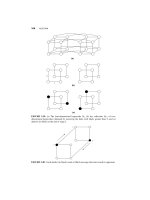
Polygons and Triangulations: Let’s consider a geometric problem that outwardly appears to be quite different from
chain-matrix multiplication, but actually has remarkable similarities. We begin with a number of definitions.
Define a polygon to be a piecewise linear closed curve in the plane. In other words, we form a cycle by joining
line segments end to end. The line segments are called the sides of the polygon and the endpoints are called the
vertices. A polygon is simple if it does not cross itself, that is, if the sides do not intersect one another except

for two consecutive sides sharing a common vertex. A simple polygon subdivides the plane into its interior, its
boundary and its exterior. A simple polygon is said to be convex if every interior angle is at most 180 degrees.
Vertices with interior angle equal to 180 degrees are normally allowed, but for this problem we will assume that
no such vertices exist.
Polygon Simple polygon Convex polygon
Fig. 10: Polygons.
Given a convex polygon, we assume that its vertices are labeled in counterclockwise order P = v
1
, ,v
n
.
We will assume that indexing of vertices is done modulo n,sov
0
=v
n
. This polygon has n sides, v
i−1
v
i
.
Given two nonadjacent sides v
i
and v
j
, where i<j−1, the line segment v
i
v
j
is a chord. (If the polygon is simple
but not convex, we include the additional requirement that the interior of the segment must lie entirely in the

interior of P .) Any chord subdivides the polygon into two polygons: v
i
,v
i+1
, ,v
j
, and v
j
,v
j+1
, ,v
i
.
Atriangulation of a convex polygon P is a subdivision of the interior of P into a collection of triangles with
disjoint interiors, whose vertices are drawn from the vertices of P . Equivalently, we can define a triangulation
as a maximal set T of nonintersecting chords. (In other words, every chord that is not in T intersects the interior
of some chord in T .) It is easy to see that such a set of chords subdivides the interior of the polygon into a
collection of triangles with pairwise disjoint interiors (and hence the name triangulation). It is not hard to prove
(by induction) that every triangulation of an n-sided polygon consists of n − 3 chords and n − 2 triangles.
Triangulations are of interest for a number of reasons. Many geometric algorithm operate by first decomposing
a complex polygonal shape into triangles.
In general, given a convex polygon, there are many possible triangulations. In fact, the number is exponential in
n, the number of sides. Which triangulation is the “best”? There are many criteria that are used depending on
the application. One criterion is to imagine that you must “pay” for the ink you use in drawing the triangulation,
and you want to minimize the amount of ink you use. (This may sound fanciful, but minimizing wire length is an
Lecture Notes 19 CMSC 451
important condition in chip design. Further, this is one of many properties which we could choose to optimize.)
This suggests the following optimization problem:
Minimum-weight convex polygon triangulation: Given a convex polygon determine the triangulation that
minimizes the sum of the perimeters of its triangles. (See Fig. 11.)

Lower weight triangulationA triangulation
Fig. 11: Triangulations of convex polygons, and the minimum weight triangulation.
Given three distinct vertices v
i
, v
j
, v
k
, we define the weight of the associated triangle by the weight function
w(v
i
,v
j
,v
k
)=|v
i
v
j
|+|v
j
v
k
|+|v
k
v
i
|,
where |v
i

v
j
| denotes the length of the line segment v
i
v
j
.
Dynamic Programming Solution: Let us consider an (n +1)-sided polygon P = v
0
,v
1
, ,v
n
. Let us assume
that these vertices have been numbered in counterclockwise order. To derive a DP formulation we need to define
a set of subproblems from which we can derive the optimum solution. For 0 ≤ i<j≤n, define t[i, j] to be the
weight of the minimum weight triangulation for the subpolygon that lies to the right of directed chord
v
i
v
j
, that
is, the polygon with the counterclockwise vertex sequence v
i
,v
i+1
, ,v
j
. Observe that if we can compute
this quantity for all such i and j, then the weight of the minimum weight triangulation of the entire polygon can

be extracted as t[0,n]. (As usual, we only compute the minimum weight. But, it is easy to modify the procedure
to extract the actual triangulation.)
As a basis case, we define the weight of the trivial “2-sided polygon” to be zero, implying that t[i, i +1]=0.
In general, to compute t[i, j], consider the subpolygon v
i
,v
i+1
, ,v
j
, where j>i+1. One of the chords of
this polygon is the side
v
i
v
j
. We may split this subpolygon by introducing a triangle whose base is this chord,
and whose third vertex is any vertex v
k
, where i<k<j. This subdivides the polygon into the subpolygons
v
i
,v
i+1
, v
k
and v
k
,v
k+1
, v

j
whose minimum weights are already known to us as t[i, k] and t[k,j].
In addition we should consider the weight of the newly added triangle v
i
v
k
v
j
. Thus, we have the following
recursive rule:
t[i, j]=

0 if j = i +1
min
i<k<j
(t[i, k]+t[k, j]+w(v
i
v
k
v
j
)) if j>i+1.
The final output is the overall minimum weight, which is, t[0,n]. This is illustrated in Fig. 12
Note that this has almost exactly the same structure as the recursive definition used in the chain matrix multipli-
cation algorithm (except that some indices are different by 1.) The same Θ(n
3
) algorithm can be applied with
only minor changes.
Relationship to Binary Trees: One explanation behind the similarity of triangulations and the chain matrix multipli-
cation algorithm is to observe that both are fundamentally related to binary trees. In the case of the chain matrix

multiplication, the associated binary tree is the evaluation tree for the multiplication, where the leaves of the
tree correspond to the matrices, and each node of the tree is associated with a product of a sequence of two or
more matrices. To see that there is a similar correspondence here, consider an (n +1)-sided convex polygon
P = v
0
,v
1
, ,v
n
, and fix one side of the polygon (say v
0
v
n
). Now consider a rooted binary tree whose root
node is the triangle containing side
v
0
v
n
, whose internal nodes are the nodes of the dual tree, and whose leaves
Lecture Notes 20 CMSC 451
k
i
k
j
n
v
j
i
v

v
v
0
v
Triangulate
at

cost

t[
i
,
k
]
at cost t[k,j]
cost=w(v ,v , v )
Triangulate
Fig. 12: Triangulations and tree structure.
correspond to the remaining sides of the tree. Observe that partitioning the polygon into triangles is equivalent
to a binary tree with n leaves, and vice versa. This is illustrated in Fig. 13. Note that every triangle is associated
with an internal node of the tree and every edge of the original polygon, except for the distinguished starting
side
v
0
v
n
, is associated with a leaf node of the tree.
v
11
1

2
3
4
5
6
7
8
9
10
root
A
6
root
v
v
v
v
v
v
v
v
v
v
v
0
A
2
A
A
4

A
71
A
5
A
8
A
A
119
A
10
A
3
9
A
8
A
7
A
6
A
5
A
2
A
1
A
4
A
3

A
11
A
10
A
Fig. 13: Triangulations and tree structure.
Once you see this connection. Then the following two observations follow easily. Observe that the associated
binary tree has n leaves, and hence (by standard results on binary trees) n − 1 internal nodes. Since each
internal node other than the root has one edge entering it, there are n −2 edges between the internal nodes. Each
internal node corresponds to one triangle, and each edge between internal nodes corresponds to one chord of the
triangulation.
Lecture 7: Greedy Algorithms: Activity Selection and Fractional Knapack
Read: Sections 16.1 and 16.2 in CLRS.
Greedy Algorithms: In many optimization algorithms a series of selections need to be made. In dynamic program-
ming we saw one way to make these selections. Namely, the optimal solution is described in a recursive manner,
and then is computed “bottom-up”. Dynamic programming is a powerful technique, but it often leads to algo-
rithms with higher than desired running times. Today we will consider an alternative design technique, called
greedy algorithms. This method typically leads to simpler and faster algorithms, but it is not as powerful or as
widely applicable as dynamic programming. We will give some examples of problems that can be solved by
greedy algorithms. (Later in the semester, we will see that this technique can be applied to a number of graph
problems as well.) Even when greedy algorithms do not produce the optimal solution, they often provide fast
heuristics (nonoptimal solution strategies), are often used in finding good approximations.
Lecture Notes 21 CMSC 451
Activity Scheduling: Activity scheduling and it is a very simple scheduling problem. We are given a set S =
{1, 2, ,n}of n activities that are to be scheduled to use some resource, where each activity must be started
at a given start time s
i
and ends at a given finish time f
i
. For example, these might be lectures that are to be

given in a lecture hall, where the lecture times have been set up in advance, or requests for boats to use a repair
facility while they are in port.
Because there is only one resource, and some start and finish times may overlap (and two lectures cannot be
given in the same room at the same time), not all the requests can be honored. We say that two activities i and
j are noninterfering if their start-finish intervals do not overlap, more formally, [s
i
,f
i
)∩[s
j
,f
j
)=∅. (Note
that making the intervals half open, two consecutive activities are not considered to interfere.) The activity
scheduling problem is to select a maximum-size set of mutually noninterfering activities for use of the resource.
(Notice that goal here is maximum number of activities, not maximum utilization. Of course different criteria
could be considered, but the greedy approach may not be optimal in general.)
How do we schedule the largest number of activities on the resource? Intuitively, we do not like long activities,
because they occupy the resource and keep us from honoring other requests. This suggests the following greedy
strategy: repeatedly select the activity with the smallest duration (f
i
− s
i
) and schedule it, provided that it does
not interfere with any previously scheduled activities. Although this seems like a reasonable strategy, this turns
out to be nonoptimal. (See Problem 17.1-4 in CLRS). Sometimes the design of a correct greedy algorithm
requires trying a few different strategies, until hitting on one that works.
Here is a greedy strategy that does work. The intuition is the same. Since we do not like activities that take a
long time, let us select the activity that finishes first and schedule it. Then, we skip all activities that interfere
with this one, and schedule the next one that has the earliest finish time, and so on. To make the selection process

faster, we assume that the activities have been sorted by their finish times, that is,
f
1
≤ f
2
≤ ≤f
n
,
Assuming this sorting, the pseudocode for the rest of the algorithm is presented below. The output is the list A
of scheduled activities. The variable prev holds the index of the most recently scheduled activity at any time, in
order to determine interferences.
Greedy Activity Scheduler
schedule(s[1 n], f[1 n]) { // given start and finish times
// we assume f[1 n] already sorted
List A = <1> // schedule activity 1 first
prev = 1
fori=2ton
if (s[i] >= f[prev]) { // no interference?
append i to A; prev = i // schedule i next
}
return A
}
It is clear that the algorithm is quite simple and efficient. The most costly activity is that of sorting the activities
by finish time, so the total running time is Θ(n log n). Fig. 14 shows an example. Each activity is represented
by its start-finish time interval. Observe that the intervals are sorted by finish time. Event 1 is scheduled first. It
interferes with activity 2 and 3. Then Event 4 is scheduled. It interferes with activity 5 and 6. Finally, activity 7
is scheduled, and it intereferes with the remaining activity. The final output is {1, 4, 7}. Note that this is not the
only optimal schedule. {2, 4, 7} is also optimal.
Proof of Optimality: Our proof of optimality is based on showing that the first choice made by the algorithm is the
best possible, and then using induction to show that the rest of the choices result in an optimal schedule. Proofs

of optimality for greedy algorithms follow a similar structure. Suppose that you have any nongreedy solution.
Lecture Notes 22 CMSC 451
4
1
4
11
Add 7:
Sched 7; Skip 8
Sched 4; Skip 5,6
Sched 1; Skip 2,3
Input:
3
2
3
2
3
5
6
2
77
5
Add 1:
7
6
7
Add 4:
8
4
8
6

5
4
2
1
3
5
8
8
6
Fig. 14: An example of the greedy algorithm for activity scheduling. The final schedule is {1, 4, 7}.
Show that its cost can be reduced by being “greedier” at some point in the solution. This proof is complicated a
bit by the fact that there may be multiple solutions. Our approach is to show that any schedule that is not greedy
can be made more greedy, without decreasing the number of activities.
Claim: The greedy algorithm gives an optimal solution to the activity scheduling problem.
Proof: Consider any optimal schedule A that is not the greedy schedule. We will construct a new optimal
schedule A

that is in some sense “greedier” than A. Order the activities in increasing order of finish
time. Let A = x
1
,x
2
, ,x
k
be the activities of A. Since A is not the same as the greedy schedule,
consider the first activity x
j
where these two schedules differ. That is, the greedy schedule is of the form
G = x
1

,x
2
, ,x
j−1
,g
j
, where g
j
= x
j
. (Note that k ≥ j, since otherwise G would have more
activities than the optimal schedule, which would be a contradiction.) The greedy algorithm selects the
activity with the earliest finish time that does not conflict with any earlier activity. Thus, we know that g
j
does not conflict with any earlier activity, and it finishes before x
j
.
Consider the modified “greedier” schedule A

that results by replacing x
j
with g
j
in the schedule A. (See
Fig. 15.) That is,
A

= x
1
,x

2
, ,x
j−1
,g
j
,x
j+1
, ,x
k
.
15
x
4
G:
x
1
x
2
A:
xx
2
x
3
x
g
3
g
3
A’:
x

1
x
2
x
4
x
5
Fig. 15: Proof of optimality for the greedy schedule (j =3).
This is a feasible schedule. (Since g
j
cannot conflict with the earlier activities, and it does not conflict with
later activities, because it finishes before x
j
.) It has the same number of activities as A, and therefore A

Lecture Notes 23 CMSC 451
is also optimal. By repeating this process, we will eventually convert A into G, without decreasing the
number of activities. Therefore, G is also optimal.
Fractional Knapsack Problem: The classical (0-1) knapsack problem is a famous optimization problem. A thief is
robbing a store, and finds n items which can be taken. The ith item is worth v
i
dollars and weighs w
i
pounds,
where v
i
and w
i
are integers. He wants to take as valuable a load as possible, but has a knapsack that can only
carry W total pounds. Which items should he take? (The reason that this is called 0-1 knapsack is that each

item must be left (0) or taken entirely (1). It is not possible to take a fraction of an item or multiple copies of an
item.) This optimization problem arises in industrial packing applications. For example, you may want to ship
some subset of items on a truck of limited capacity.
In contrast, in the fractional knapsack problem the setup is exactly the same, but the thief is allowed to take any
fraction of an item for a fraction of the weight and a fraction of the value. So, you might think of each object as
being a sack of gold, which you can partially empty out before taking.
The 0-1 knapsack problem is hard to solve, and in fact it is an NP-complete problem (meaning that there
probably doesn’t exist an efficient solution). However, there is a very simple and efficient greedy algorithm for
the fractional knapsack problem.
As in the case of the other greedy algorithms we have seen, the idea is to find the right order in which to process
items. Intuitively, it is good to have high value and bad to have high weight. This suggests that we first sort the
items according to some function that is an decreases with value and increases with weight. There are a few
choices that you might try here, but only one works. Let ρ
i
= v
i
/w
i
denote the value-per-pound ratio. We sort
the items in decreasing order of ρ
i
, and add them in this order. If the item fits, we take it all. At some point
there is an item that does not fit in the remaining space. We take as much of this item as possible, thus filling
the knapsack entirely. This is illustrated in Fig. 16
40
20 20
30
20
5
+

5 $30
$270
+
$100
$140
ρ=
40
35
5
10
20
30
40
knapsack
4.06.0 2.0 5.0 3.0
$30
60
$30 $20 $160$90$100
fractional problem.
Greedy solution to
to 0−1 problem.
Greedy solution
to 0−1 problem.
Optimal solution
Input
$100
$90
+
+
$220 $260

$160
+
$100
Fig. 16: Example for the fractional knapsack problem.
Correctness: It is intuitively easy to see that the greedy algorithm is optimal for the fractional problem. Given a room
with sacks of gold, silver, and bronze, you would obviously take as much gold as possible, then take as much
silver as possible, and then as much bronze as possible. But it would never benefit you to take a little less gold
so that you could replace it with an equal volume of bronze.
More formally, suppose to the contrary that the greedy algorithm is not optimal. This would mean that there is
an alternate selection that is optimal. Sort the items of the alternate selection in decreasing order by ρ values.
Consider the first item i on which the two selections differ. By definition, greedy takes a greater amount of item
i than the alternate (because the greedy always takes as much as it can). Let us say that greedy takes x more
Lecture Notes 24 CMSC 451
units of object i than the alternate does. All the subsequent elements of the alternate selection are of lesser value
than v
i
. By replacing x units of any such items with x units of item i, we would increase the overall value of the
alternate selection. However, this implies that the alternate selection is not optimal, a contradiction.
Nonoptimality for the 0-1 Knapsack: Next we show that the greedy algorithm is not generally optimal in the 0-1
knapsack problem. Consider the example shown in Fig. 16. If you were to sort the items by ρ
i
, then you would
first take the items of weight 5, then 20, and then (since the item of weight 40 does not fit) you would settle for
the item of weight 30, for a total value of $30 + $100 + $90 = $220. On the other hand, if you had been less
greedy, and ignored the item of weight 5, then you could take the items of weights 20 and 40 for a total value of
$100 + $160 = $260. This feature of “delaying gratification” in order to come up with a better overall solution
is your indication that the greedy solution is not optimal.
Lecture 8: Greedy Algorithms: Huffman Coding
Read: Section 16.3 in CLRS.
Huffman Codes: Huffman codes provide a method of encoding data efficiently. Normally when characters are coded

using standard codes like ASCII, each character is represented by a fixed-length codeword of bits (e.g. 8 bits
per character). Fixed-length codes are popular, because its is very easy to break a string up into its individual
characters, and to access individual characters and substrings by direct indexing. However, fixed-length codes
may not be the most efficient from the perspective of minimizing the total quantity of data.
Consider the following example. Suppose that we want to encode strings over the (rather limited) 4-character
alphabet C = {a, b, c,d}. We could use the following fixed-length code:
Character a b c d
Fixed-Length Codeword 00 01 10 11
A string such as “abacdaacac” would be encoded by replacing each of its characters by the corresponding binary
codeword.
abacdaacac
00 01 00 10 11 00 00 10 00 10
The final 20-character binary string would be “00010010110000100010”.
Now, suppose that you knew the relative probabilities of characters in advance. (This might happen by analyzing
many strings over a long period of time. In applications like data compression, where you want to encode one
file, you can just scan the file and determine the exact frequencies of all the characters.) You can use this
knowledge to encode strings differently. Frequently occurring characters are encoded using fewer bits and less
frequent characters are encoded using more bits. For example, suppose that characters are expected to occur
with the following probabilities. We could design a variable-length code which would do a better job.
Character a b c d
Probability 0.60 0.05 0.30 0.05
Variable-Length Codeword 0 110 10 111
Notice that there is no requirement that the alphabetical order of character correspond to any sort of ordering
applied to the codewords. Now, the same string would be encoded as follows.
abac daacac
01100101110010010
Lecture Notes 25 CMSC 451