Mapping WGMs of erbium doped glass microsphere using near-field optical probe
Bạn đang xem bản rút gọn của tài liệu. Xem và tải ngay bản đầy đủ của tài liệu tại đây (1.58 MB, 79 trang )
1
Vietnam national university, Hanoi
College of Technology
Ho Duc Vinh
Mapping WGMs of
Erbium doped glass microsphere using
Near-field optical probe
Mapping WGMs of
Erbium doped glass microsphere using
Near-field optical probe
Master thesis
Supervisor: Dr. Tran Thi Tam
Click to buy NOW!
P
D
F
-
X
C
H
A
N
G
E
w
w
w
.
d
o
c
u
-
t
r
a
c
k
.
c
o
m
Click to buy NOW!
P
D
F
-
X
C
H
A
N
G
E
w
w
w
.
d
o
c
u
-
t
r
a
c
k
.
c
o
m
CONTENT
1. INTRODUCTION
2. CHAPTER I: MORPHOLOGY DEPENDENT RESONANCES
3. CHAPTER II: COUPLING MICROSPHERES WGMs BASED ON
NEAR-FIELD OPTICS
4. CHAPTER III: FABRICATION OF MICROSPHERE AND TAPER
FIBER
5. CHAPTER IV: EXPERIMENTS AND RESULTS
CONCLUSION
Chapter 1
Morphology Dependent Resonances
Ho Duc Vinh
K10N
5
chapter 1: Morphology Dependent Resonances
(MDRs-WGMs)
1.1. Dielectric Microsphere - A simple Model of WGMs:
Microspheres act as high Q resonators in optical regime. The curved surface
of a microshere leads to efficient confinement of light waves. The light waves
totally reflect at the surface and propagate along the circumference. If they round in
phase, resonant standing waves are produced near the surface. Such resonances are
called "morphology dependent resonances (MDRs)" because the resonance
frequencies strongly depend on the size parameter
λ
π
a
x
2
=
, (where a is the radius of
microstructure and
λ
is the light wavelength). Alternatively , the resonant modes
are often called "Whispering Gallery Modes (WGMs)". The WGMs are named
because of the similarity with acoustic waves traveling around the inside wall of a
gallery. Early this century, L.Rayleigh [46] first observed and analyzed the
"whispers" propagating around the dome of St.Catherine's cathedral in England.
Optical processes associated with WGMs have been studied extensively in recent
years [45].
WGMs are characterized by three numbers, n, l and m, for both polarizations
corresponding to TE (transverse electric) and TM (transverse magnetic) modes. TE
and TM modes have no radial components of electric and magnetic fields,
respectively. These integers distinguish intensity distribution of the resonant mode
inside a microsphere (a simple model system of Micro resonators). The order
number n indicates the number of peaks in the radial intensity distribution inside the
sphere and the mode number l is the number of waves of resonant light along the
circumference of the sphere. The azimuthal mode number m describes azimuthal
spatial distribution of the mode. For the perfect sphere, modes of WGMs are
degenerate in respect to m.
In this section, firstly, it presents a simple model of WGMs in terms ray and
wave optics for a qualitative interpretation.
Click to buy NOW!
P
D
F
-
X
C
H
A
N
G
E
w
w
w
.
d
o
c
u
-
t
r
a
c
k
.
c
o
m
Click to buy NOW!
P
D
F
-
X
C
H
A
N
G
E
w
w
w
.
d
o
c
u
-
t
r
a
c
k
.
c
o
m
Chapter 1
Morphology Dependent Resonances
Ho Duc Vinh
K10N
6
1.1.1 Ray and Wave Optics Approach:
The most intuitive picture describing the optical resonances of microsphere is
based upon ray and wave optics.
* Ray optics:
Consider a microsphere with radius a and a refractive index
()
n
ω
, and a ray
of light propagating inside, hitting the surface with angle of incidence
in
θ
(Figure
1.1.a).
Figure 1.1. a/ Ray at glancing angle is totally reflected
b/ If optical path = integral number of wavelengths, a resonance is formed
If
arcsin(1/ ( ))
inc
n
θθω
>=
, then total internal reflection occurs. Because of
spherical symmetry, all subsequent angles of incidence are the same, and the ray is
trapped. Leakage occurs only through diffractive effects, i.e., because of the
finiteness of
λ
/a
, where
λ
is the wavelength in vacuum. The leakage is expected to
be exponentially small. This simple geometric picture leads to the concept of
resonances. For large microspheres ( a >>
λ
), the trapped ray propagates close to
the surface, and traverses a distance
a
π
2
≈
in one round trip [52]. If one round trip
exactly equals l wavelengths in the medium (l = integer), then a standing wave can
occur (Figure 1.1 b).This condition translates into
2
()
a
n
λ
π
ω
≈ l
(1.1)
A dimensionless size parameter x is defined for this system
λ
π
a
x
2
=
(1.2)
cinc
θθ
>
Inphase
Click to buy NOW!
P
D
F
-
X
C
H
A
N
G
E
w
w
w
.
d
o
c
u
-
t
r
a
c
k
.
c
o
m
Click to buy NOW!
P
D
F
-
X
C
H
A
N
G
E
w
w
w
.
d
o
c
u
-
t
r
a
c
k
.
c
o
m
Chapter 1
Morphology Dependent Resonances
Ho Duc Vinh
K10N
7
In terms of which the resonance condition is
()
x
n
ω
≈
l
(1.3)
Consider the ray in Figure 1.1.a as a photon. Its momentum is
[2 ( / ( ))]
pkn
πλω
==
hh
(1.4)
where p is the momentum of photons,
h
is the Planck’s constant divided by
π
2
, and
k is the wave number. If this ray strikes the surface at near-glancing incidence
(
2
πθ
≈
in
), then the angular momentum, denoted as
h
l
, is
2 ( / ( ))
apan
πλω
≈=
hh
l
(1.5)
which is identical to Equation 1.3. The point of this derivation is to identify the
integer
l
, originally introduced as the number of wavelengths in the circumference,
as the angular momentum in the usual sense.
The great-circle orbit of the rays need not be confined to the x-y plane (e.g.,
the equatorial plane). If the orbit is inclined at an angle
θ
with respect to the z-axis,
the z-component of the angular momentum of the mode is (see Figure. 1.2)
.cos()
2
m
π
θ
=−
l
(1.6)
For a perfect sphere, all of the m modes are degenerate (with 2
l
+1
degeneracy). The degeneracy is partially lifted when the cavity is axisymmetrically
(along the z-axis) deformed from sphericity. For such distortions the integer values
for m are
, ( 1), 0,
±±−
ll
where the degeneracy remains, because the resonance
modes are independent of the circulation direction (clockwise or counterclockwise)
[49]. Highly accurate measurements of the clockwise and counterclockwise
circulating m-mode frequencies reveal a splitting due to internal backscattering, that
couples the two counter propagating modes [47].
Geometrical interpretation of light interaction with a microsphere has several
limitations:
- It cannot explain escape of light from a WGM (for perfect spheres), and
hence the characteristic leakage rates cannot be calculated.
Click to buy NOW!
P
D
F
-
X
C
H
A
N
G
E
w
w
w
.
d
o
c
u
-
t
r
a
c
k
.
c
o
m
Click to buy NOW!
P
D
F
-
X
C
H
A
N
G
E
w
w
w
.
d
o
c
u
-
t
r
a
c
k
.
c
o
m
Chapter 1
Morphology Dependent Resonances
Ho Duc Vinh
K10N
8
- Geometric optics provides no possibility for incident light to couple into a
WGM.
- The polarization of light is not taken into account.
- The radial character of the optical modes cannot be determined by
geometrical optics [7].
* Wave optics:
The proper description of the system should reply on Maxwell’s equations,
which, for a definite frequency ω and in units where C = 1, is
(
)
(
)
0
2
=−×∇×∇ ErE
εω
(1.7)
Here we assume that the dielectric constant ε depends only on the radius a,
i.e., the system is spherically symmetric. The transverse electric (TE) modes are
characterized by
(
)
(
)
(
)
,
mm
Er aX
θ
=ΦΦ
ll
(1.8)
where
( )
1/2
1
mm
X LY
−
=+
ll
ll
is the vector spherical harmonic and
L ai
= ×∇
. The
waves are then described by a scalar equation [19]
()
(
)
2
2
2
1
0
d
a
daa
ωε
−
Φ
+ − Φ=
ll
(1.9)
where the scalar function
Φ
is related to the radial function of the field as
(
)
m
aa
φ
Φ=
l
(1.10)
similarly, the transverse magnetic (TM) modes are characterized by
()
()
()
1
mm
Er aX
a
φ
ε
= ∇×
ll
(1.11)
and is again reducible to a scalar equation [19]
()
(
)
()
2
2
1
1
0
dd
da a da a a
ω
εε
+
Φ
+ − Φ=
ll
(1.12)
where in this case the scalar function is again given by (1.10). Hence, the radial
character of the optical modes could be determined by wave optics.
Click to buy NOW!
P
D
F
-
X
C
H
A
N
G
E
w
w
w
.
d
o
c
u
-
t
r
a
c
k
.
c
o
m
Click to buy NOW!
P
D
F
-
X
C
H
A
N
G
E
w
w
w
.
d
o
c
u
-
t
r
a
c
k
.
c
o
m
Chapter 1
Morphology Dependent Resonances
Ho Duc Vinh
K10N
9
1.1.2 Lorenz-Mie Theory:
A complete description of the interaction of light with a dielectric is given by
electromagnetic theory which is solved basically in wave optics above. The spherical
geometry suggests expanding the fields in terms of vector spherical harmonics.
Characteristic equations for the WGMs are derived by requiring continuity of the
tangential components of both the electric and magnetic fields at the boundary of
the dielectric sphere and the surrounding medium. Internal intensity distributions
are determined by expanding the incident wave (plane-wave of focused beam),
internal field, and external field, all in terms of vector spherical harmonics and again
imposing appropriate boundary conditions.
Figure 1.2: The resonant light wave propagates along the great circle whose normal
direction is inclined at an angle
2
πθ
−
with respect to the z-axis.
The WGMs of a microsphere are analyzed by the localization principle and
the Generalized Lorenz-Mie Theory (GLMT) [36, 34, 51]. Therefore, each WGM is
characterized by a mode order n , a mode number
l
and an azimuthal mode m,
which are described above and are summarized here:
+ The radial mode order n indicates the number of maxima in the internal
electric field distribution in the radial direction.
+ The mode number
l
gives the number of maxima between 0
o
and 180
o
degrees in the angular distribution of the energy of the WGM.
+ Each mode WGM of the microsphere also has an azimuthal angular
dependence from 0
o
and 360
o
, which is define with an azimuthal mode number m.
Click to buy NOW!
P
D
F
-
X
C
H
A
N
G
E
w
w
w
.
d
o
c
u
-
t
r
a
c
k
.
c
o
m
Click to buy NOW!
P
D
F
-
X
C
H
A
N
G
E
w
w
w
.
d
o
c
u
-
t
r
a
c
k
.
c
o
m
Chapter 1
Morphology Dependent Resonances
Ho Duc Vinh
K10N
10
However, for sphere, WGMs differing only in azimuthal mode number have
identical resonance frequencies.
The characteristic eigenvalue equations for the natural resonant frequencies
of dielectric microsphere have been solved in homogeneous surroundings. WGMs
correspond to solutions of these characteristic equations of the electromagnetic
fields in the presence of a sphere. The characteristic equations are obtained by
expanding the fields in vector spherical harmonics and then matching the tangential
components of the electric and magnetic fields at the surface of the sphere. No
incident field is assumed in deriving the characteristic equations [17].
For modes having no radial component of the magnetic field (transverse
magnetic or TM modes) the characteristic equation is,
[ ]
'
'
(1)
2 (1)
()
() (())
( ) (( )) ()
xhx
njnx
n jn x hx
ωω
ωω
=
l
l
ll
(1.13)
where x is the size parameter,
λ
π
a
x
2
=
, a is the radius,
λ
is the wavelength, and
()
n
ω
is the ratio of the refractive index of dielectric microsphere to that of the
surrounding medium.
The characteristic equation for modes having no radial component of the
electric field (transverse electric or TE modes) is:
[ ]
'
'
(1)
(1)
()
() (())
(())
()
xhx
nxjnx
jnx
hx
ωω
ω
=
l
l
l
l
(1.14)
The characteristic equations are independent of the incident field. In equation
1.13 and equation 1.14, j
l
(x) and h
l
(1)
(x) are the spherical Bessel and the Hankel
functions of the first kind, respectively. The prime (‘) denotes differentiation with
respect to the argument. The transcendental equation is satisfied only by a discrete
set of characteristic values of the size parameter, x
n,l
, corresponding to the radial n
th
root for each angular l.
The elastically scattered field can be written as an expansion of vector
spherical wave functions with TE coefficients (a
l
) and TM coefficients (b
l
) for a
Click to buy NOW!
P
D
F
-
X
C
H
A
N
G
E
w
w
w
.
d
o
c
u
-
t
r
a
c
k
.
c
o
m
Click to buy NOW!
P
D
F
-
X
C
H
A
N
G
E
w
w
w
.
d
o
c
u
-
t
r
a
c
k
.
c
o
m
Chapter 1
Morphology Dependent Resonances
Ho Duc Vinh
K10N
11
plane wave incident on a dielectric microsphere. The scattered field becomes infinite
at complex frequencies
(,)
n
ω
l
corresponding to the complex size parameters x
(n,l)
, at
which, a
l
and b
l
become infinite.
Fig. 2.3: Three light waves; the linearly polarized incident plane wave, the spherical
wave inside the sphere and the spherical wave scattered by the sphere.
a
l
coefficients are associated with TE
n,l
WGMs specified by:
[
]
[
]
[ ]
''
2
'
'
(2) 2 (2)
() () (()) () (()) ()
() () (()) () (()) ()
jxn xjn x n jn xxjx
a
hxnxjnx n jnxxhx
ω ω ωω
ω ω ωω
−
=
−
ll ll
l
l l ll
(1.15)
Similarly, b
l
coefficients are associated with the TM
n,l
WGMs as specified by
equation 1.16, where
(2)
()
hx
l
are the spherical Hankel functions of the second type
[6].
[
]
[
]
[ ]
''
'
'
(2) (2)
() () (()) (()) ()
() () (()) (()) ()
jxnxjnx jnxxjx
b
hxnxjnx jnxxhx
ωωω
ωωω
−
=
−
ll ll
l
l l ll
(1.16)
The WGMs of the microsphere occur at the zeros of the denominators (or
poles) of a
l
and b
l
coefficients. These complex poles occur at discrete values of the
complex size parameter x. The modes are radiative for real frequencies, and hence
the modes are virtual when the resonance frequencies are complex.
+ The real part of the pole frequency is close to real resonance frequency
[19].
+ The imaginary part of the pole frequency determines the linewidth of the
resonance [37].
Click to buy NOW!
P
D
F
-
X
C
H
A
N
G
E
w
w
w
.
d
o
c
u
-
t
r
a
c
k
.
c
o
m
Click to buy NOW!
P
D
F
-
X
C
H
A
N
G
E
w
w
w
.
d
o
c
u
-
t
r
a
c
k
.
c
o
m
Chapter 1
Morphology Dependent Resonances
Ho Duc Vinh
K10N
12
For a fixed radius, the WGMs have
l
values that are bound by
()
x nx
ω
<<
l
[28] (see equation 1.3), where the upper limit is the maximum number of
wavelengths that fit inside the circumference. The radial electric field distribution of
the lowest order modes (n
th
) shows a peak just inside the surface. The higher the
mode order becomes, the more the mode distribution goes to inner region [30].
For larger size parameters the first order resonances become narrow while the
higher order resonances heighten and become dominant [8].
The first peaks observed in the spectra are the first-order resonances. The
second order resonances begin to appear when the size parameter increases due to
decreasing the linewidths. As the size parameter increases further, the linewidths of
the first and second order resonances decrease further and third-order resonances
begin to appear.
The natural resonance frequencies associated with the TE
n,l
and TM
n,l
modes
are given by equation 1.17, where
µ
is the permeability and
ε
permittivity of the
surrounding lossless medium [23]. Thus, equation 1.17 definitions the complex
frequencies at which a dielectric sphere will resonate in one of its natural modes are:
,
,
n
n
x
a
ω
µε
=
l
l
(1.17)
Figure 1.3. WGM mode spacing
λ
∆
and the WGM linewidth
2/1
λ
Based on the Lorenz-Mie theory, the separation between the adjacent peak
wavelengths of the same mode order (n) WGMs with subsequent mode numbers
λ
∆
2/1
λ
Wavelength
Mode Density (a.u.)
Click to buy NOW!
P
D
F
-
X
C
H
A
N
G
E
w
w
w
.
d
o
c
u
-
t
r
a
c
k
.
c
o
m
Click to buy NOW!
P
D
F
-
X
C
H
A
N
G
E
w
w
w
.
d
o
c
u
-
t
r
a
c
k
.
c
o
m
Chapter 1
Morphology Dependent Resonances
Ho Duc Vinh
K10N
13
(
l
), mode spacing (
λ
∆
), is approximately given by Eq. 1.18. The full width at half
maximum (FWHM) of the resonance or the resonance linewidth are denoted by
2/1
λ
,
see Fig. 1.3 [57]
22
2
arctan( ( ) 1)
2 ()1
n
an
λω
λ
πω
−
∆=
−
(1.18)
1.2. Characteristics of Dielectric Microsphere:
1.2.1. WGM Position:
For spheres with large x, several expressions are derived to determine the
spectral location, separation, and width of WGMs. The positions of WGMs are
approximated by [26, 10]:
1322
13 13 23 2 13 23 33
,
3
3 2 ( ( ) 2 3)
() 2 (2) ()
10
nnnn
P PnP
n x v v v v Ov
ω
ωααα
ρρ
−
− −− −−
−
=+−+−+
l
(1.19)
where
()
Pn
ω
=
for TE modes,
1/()
Pn
ω
=
for TM modes,
1/2
v
=+
l
,
22
()1
n
ρω
=−
,
n
α
are the roots of the Airy function, and
3
()
i
O
ν
−
are the i
th
fractional
forms of the Airy function .
1.2.2. WGM Separation:
The separation between resonances
,
n
x
∆
l
is more useful than the absolute
mode positions to determine the approximate sphere size and approximating mode
numbers. Asymptotic analysis gives:
13 23
23 2 43
,
22
()1
3 10
n nn
nx vv
ω αα
−−
−−
∆=+−
l
2223 13
532
4/3
( ( ) 2 3)22
()
39
n
PnP
v Ov
ω
α
ρ
−
−−
−
+ −+
(1.20)
Although equation 1.20 is more accurate, a simple approximation to
x
∆
is
given by:
Click to buy NOW!
P
D
F
-
X
C
H
A
N
G
E
w
w
w
.
d
o
c
u
-
t
r
a
c
k
.
c
o
m
Click to buy NOW!
P
D
F
-
X
C
H
A
N
G
E
w
w
w
.
d
o
c
u
-
t
r
a
c
k
.
c
o
m
Chapter 1
Morphology Dependent Resonances
Ho Duc Vinh
K10N
14
1/2
12
1/2
2
tan(()/)1
(()/)1
nx
x
nx
ω
ω
−
−
∆=
−
l
ll
for
1/2
x −
?
l (1.21a)
1
tan
x
ρ
ρ
−
∆=
for x/l =1 (1.21b)
1.2.3. WGM Density:
An approximation to the mode density of high-Q WGMs, which is defined as
the number of resonance modes per frequency or size-parameter interval, is [50]:
WGM Density
(
)
21
tanx
ρρρ
π
−
−
=
(1.22)
Equation 1.22 implies that the mode density increases rapidly as the refractive index
increases.
1.2.4. Spatial Distribution of WGMs:
Spatial characteristics of WGMs are described in terms of M and N at
resonant size parameters satisfying the characteristic equations. Since TE modes are
defined as the electric field having no radial components, these modes are
represented by the vector functions M. Similarly, since TM modes are defined as the
magnetic field having no radial components, these modes are represented by the
vector functions N. The corresponding electric fields are represented by the vector
functions N because the rotation of M is proportional to N.
Using the vector wave functions, the internal electric fields of a sphere are
expanded as a sum of electric fields (TE modes and one of TM modes). The spatial
distributions of the electric field of TE and TM modes of WGMs are obtained
by
2
TE
E
and
2
TM
E
at the size parameter satisfying characteristic equations for a
given
l
.
Figure 1.4 shows the internal intensity distributions in the equatorial plane of
a sphere with index of refraction ratio n(
ω
) = 1,4 for (A) TE
30,1
, (B) TE
30,2
, and
(C)TE
30,3
modes, where the subscript denote angular mode and the order numbers.
The resonant size parameter is shown in the upper side of each figure. Here the
Click to buy NOW!
P
D
F
-
X
C
H
A
N
G
E
w
w
w
.
d
o
c
u
-
t
r
a
c
k
.
c
o
m
Click to buy NOW!
P
D
F
-
X
C
H
A
N
G
E
w
w
w
.
d
o
c
u
-
t
r
a
c
k
.
c
o
m
Chapter 1
Morphology Dependent Resonances
Ho Duc Vinh
K10N
15
distributions are obtained by adding WGMs rounding along the +
Φ
(m = 30) and -
Φ
(m = -30) directions. Remarkably, the number of peaks in the angular distribution
is identical as the mode number l multiplied by a factor 2 (l from 0
o
to 180
o
), while
the number of peaks in the radial intensity is the mode order n.
Figure 1.4. The internal intensity distributions in the equatorial plane for
(A)TE
30,1
, (B)TE
30,2
and (C)TE
30,3
modes of a sphere with n(ω) = 1,4. The resonant
size parameters are shown in the upper side of each figure.
As the mode order increases, number of peaks in the internal intensity profile
increases, corresponding to the mode order, and the highest peak is located at the
most inner side in the radial direction. An illustration of the angle-averaged radial
intensity distribution for the same mode number with n=1,2,3 is shown in
figure.1.5.(A).
Click to buy NOW!
P
D
F
-
X
C
H
A
N
G
E
w
w
w
.
d
o
c
u
-
t
r
a
c
k
.
c
o
m
Click to buy NOW!
P
D
F
-
X
C
H
A
N
G
E
w
w
w
.
d
o
c
u
-
t
r
a
c
k
.
c
o
m
Chapter 1
Morphology Dependent Resonances
Ho Duc Vinh
K10N
16
Fig 1.5. (A) Typical illustration of angle-averaged intensity distribution profile
along the radial direction for WGMs n=1,2,3 with same l.
(B) ) Typical illustration of internal-intensity distribution as
a function of θ for TE WGMs with m = 1, l/2, and l.
Figure1.6. The internal intensity distribution as a function of θ for TE WGMs with
l=30, and m=1, 15, and 30. The maximum intensity of each m-mode
is located near
1
sin( /)
m
θ
−
=
l
The dependence of the internal intensity distribution on the azimuthal mode
number m is depicted in figure 1.5(B), in which the angular internal intensity
distribution is a function of
θ
. Three WGMs for m=1, l/2 and l are illustrated as the
angle
θ
varies from 0
o
to 90
o
. These WGMs have the same resonance frequency, but
A B
Click to buy NOW!
P
D
F
-
X
C
H
A
N
G
E
w
w
w
.
d
o
c
u
-
t
r
a
c
k
.
c
o
m
Click to buy NOW!
P
D
F
-
X
C
H
A
N
G
E
w
w
w
.
d
o
c
u
-
t
r
a
c
k
.
c
o
m
Chapter 1
Morphology Dependent Resonances
Ho Duc Vinh
K10N
17
the maximum intensity for each m is inclined at an angle
1
sin( /)
m
θ
−
=
l
. The
maximum intensity peak agrees with the ray optics picture of an m-mode circulating
in a confined orbit inclined at
1
sin( /)
m
θ
−
=
l
and with its normal inclined at an angle
1
cos( /)
m
θ
−
=
l
.
Figure 1.6. shows the angular distribution of three TE WGMs with l = 30 and
m = 1, 15 and 30 as a function of
θ
varied form 0 to 90 degrees. The maximum
intensity of each m mode is located near
1
sin( /)
m
θ
−
=
l
. The m = 1 mode is
confined near the pole region. The m = 15 mode is located near
1
sin (15/30) 30
o
θ
−
==
and the m = 30 mode is near the equatorial plane (
90
o
θ
=
).
These results are consistent with the qualitative interpretation mentioned in the
previous subsection although the spatial distributions shown in this figure have
somewhat broader structure.
1.2.5. Resonator Quality of Microsphere WGMs:
Based on the theory of electromagnetic fields, the quality factor-Q of a
resonance is defined as:
,,
,
,,
Re()
2Im()
nn
n
nn
x
Q
x
ω
ωτ
ω
= ==
∆
ll
l
ll
(1.23)
where
τ
is the life time of a wave on a WGM. In a perfectly smooth homogeneous
lossless sphere the Q values are limited by diffractive leakage losses and can be as
high as 10
10
. In reality, volume inhomogeneities, surface roughness, and absorption
restrict the maximum Q values to be less than 10
10
. Local or global shape
deformations and nonlinear effects can further reduce the maximum Q value.
For frequencies near a WGM, the electric field inside the cavity varies as:
)
2
exp()(
0
00
t
Q
tiEtE
ω
ω
−−=
(1.24)
The decay term leads to a broadening of the resonance linewidth, giving a
Lorentzian lineshape for the energy distribution
2
0
2
0
2
)2()(
1
|)(|
Q
E
ωωω
ω
+−
∝
(1.25)
Click to buy NOW!
P
D
F
-
X
C
H
A
N
G
E
w
w
w
.
d
o
c
u
-
t
r
a
c
k
.
c
o
m
Click to buy NOW!
P
D
F
-
X
C
H
A
N
G
E
w
w
w
.
d
o
c
u
-
t
r
a
c
k
.
c
o
m
Chapter 1
Morphology Dependent Resonances
Ho Duc Vinh
K10N
18
Figure 1.7. The angle average intensity as a function of the normalized radius r/a for
TE WGMs with l=60, and n=1, 2, 3. The refractive index of microsphere is 1.4
When resonant standing waves grow inside a sphere, the spherical particle
acts as a high Q resonator. A fraction of the resonant light wave leaks due to the
diffractive effect and the quality factor Q of the resonator is limited by the
diffractive losses. The electric fields of the WGMs extend beyond the particle
boundary as evanescent waves. The lowest order WGM has the maximum of the
internal distribution at the region nearest the surface of the sphere, and has the
shortest penetration depth toward the outer region of the sphere. For a given mode
number l, the n=1 modes have the highest Q (smallest ∆x), with a peak intensity
located closest to the surface and the evanescent wave penetrating shortest into the
surrounding medium. As n increases, the Q value decreases, the peak intensity
moves away from the surface, and the evanescent wave penetration into the
surrounding medium increases. For a fixed radial mode order n, modes with higher
angular momentum or higher mode number l have higher Q values. Figure 1.7
shows the angle averaged intensity as a function of the normalized radius r/a for TE
WGMs with
l
= 60 and n = 1, 2 and 3. The refractive index of the sphere is 1.4.
This result is obtained by computing
2
TE
E
integrated over the total solid angle [42].
Click to buy NOW!
P
D
F
-
X
C
H
A
N
G
E
w
w
w
.
d
o
c
u
-
t
r
a
c
k
.
c
o
m
Click to buy NOW!
P
D
F
-
X
C
H
A
N
G
E
w
w
w
.
d
o
c
u
-
t
r
a
c
k
.
c
o
m
Chapter 1
Morphology Dependent Resonances
Ho Duc Vinh
K10N
19
Figure 1.8: The resonance curves for the same WGMs and the sphere as in Fig.1.7
as a function of the size parameter, where each x
0
is centered.
TE
60,1
TE
60,2
TE
60,3
Resonance size parameter 47.491 51.677 55.218
Quality factor 9.4 x 10
6
3.9 x 10
4
1.6 x 10
3
Table.1: The resonance size parameters and the quality factors of TE MDRs
with
l
= 60 and n = 1, 2 and 3.
Figure 1.8 shows the resonance curves for the same WGMs and sphere as in
Figure 1.7 as a function of the size parameter, where each resonant size parameter x
o
is centered. The resonance curve of the lowest order WGM is extremely narrow
compared with the higher order WGMs. The quality factor Q of the WGM can be
also defined as:
0
x
Q
x
=
∆
(1.26)
where
x
∆
is the full width at the half maximum of the resonance curve. The
resonance size parameters and the quality factors of these modes are summarized in
Table.1. The lowest order WGM with the same mode number has the highest quality
factor and is therefore most strongly confined inside the sphere.
Click to buy NOW!
P
D
F
-
X
C
H
A
N
G
E
w
w
w
.
d
o
c
u
-
t
r
a
c
k
.
c
o
m
Click to buy NOW!
P
D
F
-
X
C
H
A
N
G
E
w
w
w
.
d
o
c
u
-
t
r
a
c
k
.
c
o
m
Chapter 1
Morphology Dependent Resonances
Ho Duc Vinh
K10N
20
Figure 1.9: the resonance curves for the first order TE MDRs with
l
= 30, 45 and
60 as a function of the size parameter x
0
is also centered. The refractive index of the
sphere is 1.4.
Table.2: The resonance size parameters and the quality factors of the first
order TE WGMs with
l
= 30, 45 and 60.
TE
30,1
TE
45,1
TE
60,1
Resonance size parameter 24.969 36.299 47.491
Quality factor 2.3 x 10
3
1.3 x 10
5
9.4 x 10
6
Figure 1.9 shows the resonance curves for the first order TE WGMs with
l
=
30, 45 and 60 as a function of the size parameter, where x
0
is also centered. The
refractive index of the sphere is 1.4. Q increases as the mode number is increased
for a fixed n. The resonance curve of TE
60,1
WGM is also extremely narrow
compared with the lower mode WGMs. The resonance size parameters and the
quality factors of these modes are summarized in Table.2.
On the other hand, one can describe the performance of a resonator element
in terms of its capacity to store energy. The quality factor (Q-factor) determines how
long a photon can be stored inside a WGM [18]. Therefore the quality (Q) of a
resonance is governed by the losses associated with it. The observed resonator
quality is the geometric sum of the qualities of each mechanism.
couplingobserved
QQQ
111
0
+=
(1.27)
Click to buy NOW!
P
D
F
-
X
C
H
A
N
G
E
w
w
w
.
d
o
c
u
-
t
r
a
c
k
.
c
o
m
Click to buy NOW!
P
D
F
-
X
C
H
A
N
G
E
w
w
w
.
d
o
c
u
-
t
r
a
c
k
.
c
o
m
Chapter 1
Morphology Dependent Resonances
Ho Duc Vinh
K10N
21
Alternatively, the observed spectral width is the sum of the widths of all the
different loss mechanisms. The internal losses (Q
0
) are composed of absorption
losses (Q
abs
), diffraction leakage losses (Q
r
) and scattering losses (Q
s
) .The external
loss is due to coupling (Q
coupling
).
srabs
QQQQ
1111
0
++=
(1.28)
In an optical microsphere WGM resonator, energy storage may be thought of as the
retention of individual light rays that have been inserted into the cavity [15]. The
value of the quality factor roughly equals the number of times a given ray can be
expected to travel around the sphere before succumbing to a loss process. In silica
microspheres, internal loss effects include scattering from surface irregularities,
absorption due to molecular resonances, Rayleigh scattering. Surface scattering is
extremely low, since extremely smooth surfaces can be fabricated. Therefore,
absorption and Rayleigh scattering dominate the losses [30].
1.2.6. Mode volume of microsphere WGMs:
In many applications, not only temporal confinement of light (i.e. the Q-
factor), but also the spatial extension to which the light is confined is an important
performance parameter. Several definitions of mode volume can be encountered in
literature, and are discussed in this section. The most common definition of mode
volume is related to the definition of the energy density of the optical mode.
It is defined as the equivalent volume, the mode occupies if the energy density
was distributed homogeneously throughout the mode volume, at the peak value:
() ()
BBEErr
me
µ
+ε=ϖ+ϖ
2
1
2
1
(1.29)
() ()
(
)
() ()
( )
() ()
() ()
(
)
2
3
2
max
max
em
Mode
em
r r dV r Er dr
V
rr
r Er
ϖϖε
ϖϖ
ε
+
==
+
∫∫
r
r
(1.30)
The mode volumes using these formulas can be well approximated by:
( )
( )
≅
TMnD
TEnD
V
spherem
67611
67611
081
021
//
//
,
/.
/.
λ
λ
(1.31)
Click to buy NOW!
P
D
F
-
X
C
H
A
N
G
E
w
w
w
.
d
o
c
u
-
t
r
a
c
k
.
c
o
m
Click to buy NOW!
P
D
F
-
X
C
H
A
N
G
E
w
w
w
.
d
o
c
u
-
t
r
a
c
k
.
c
o
m
Chapter 2
Coupling Microsphere WGMs based on near-field optics
Ho Duc Vinh
K10N
22
Chapter 2: Coupling Microsphere WGMs based on
Near-field Optics
2.1. Introduction of Near-field optics
Near-field optics has developed very rapidly from around the middles 1980s
after preliminary trials in the microwave frequency region, as proposed as early as
1928. At the early stages of this development, most technical efforts were devoted to
realizing super-high-resolution optical microscopy beyond the diffraction limit.
However, the possibility of exploiting the optical near-field, phenomenon of
quasistatic electromagnetic interaction at subwavelength distances between
nanometric particles has opened new ways to nanometric optical science and
technology, and many applications in the field of nanometric fabrication and
manipulation have been proposed and implemented. For optical telecommunication
system, near-field optics can demonstrate lots of photonic phenomena such as
quantum electrodynamics (QED), CQED… And one of spectacular examples is
near-field interaction of microcavities and tip guide. It is my purpose to use a simple
and practical theory so that we can understand easily the fundamental physics of the
near-field in three dimensions and to obtain a general expression for each field
component which will serve as a guide to more complicated cases. This part will
show that the analytic forms of the near-field components around a microsphere
produced by an incident plane wave can be obtained and that the effect of near-field
can be evaluated in some applications. Comparison of our theory with an
experimental result reported by other authors shows good agreement. It will also
verify that the localization area of the near field is proportional to the size of the
microsphere, and that the field momentum is locally modified by the interference
between the near field and the incident field and that the modulation amount is
dependent on the size of the sphere, instead of the wavelength of the light. Also, It
could be seen the relationship of Evanescent-field with Near-field optics and the
scope of near-field optics in the modern optical telecommunication depicted
hereinafter.
Click to buy NOW!
P
D
F
-
X
C
H
A
N
G
E
w
w
w
.
d
o
c
u
-
t
r
a
c
k
.
c
o
m
Click to buy NOW!
P
D
F
-
X
C
H
A
N
G
E
w
w
w
.
d
o
c
u
-
t
r
a
c
k
.
c
o
m
Chapter 2
Coupling Microsphere WGMs based on near-field optics
Ho Duc Vinh
K10N
23
Figure 2.1 Near-field optics and related problems. Optical processes are
shown in terms of the scales given by the size of the material object and the spatial
extent of the effective field.
2.2.
Evanescent coupling techniques for optical micro-cavities:
The study of the optical properties of ultra-high-Q (UHQ) microcavities
requires the ability to optically excite and probe the resonator. Furthermore, the
investigation of the full potential of UHQ structures to realize high performance
devices, such as low-loss passive elements and low-threshold active elements such
as nonlinear sources, requires an ability to both efficiently excite the modes of the
cavity and to efficiently extract optical energy from the cavity. There are several
commonly used techniques to couple optical microcavities. These fall into two
classes: phase-matched and non-phase-matched techniques. Of the two, phase-
matched schemes offer a dramatic advantage in terms of coupling efficiency both
into and out-of the cavity, relegating non-phase-matched schemes (of which free-
space illumination is the sole member) to systems where experimental limitations
Spatial Extent
of
Effective Field
or
Sample-Probe
Distance
Propagating Light Wave
Cavity QED
Photon
Localiztion
Optical Property
of Mesoscopic
Material System
Optical Near Field
Photon-
Assisted
Tunneling &
Light
Emission
From STM
NOM
& Relatives
Functional Probe SPM
& Elementary Excitation STM
Material Excitation
Single Exciton
Tunneling &
Probing
Sizeof Matter
100 nm
1
µ
m
1
µ
m
100 nm
10 nm
10 nm
1 nm
1 nm
0.1 nm
0.1 nm
Click to buy NOW!
P
D
F
-
X
C
H
A
N
G
E
w
w
w
.
d
o
c
u
-
t
r
a
c
k
.
c
o
m
Click to buy NOW!
P
D
F
-
X
C
H
A
N
G
E
w
w
w
.
d
o
c
u
-
t
r
a
c
k
.
c
o
m
Chapter 2
Coupling Microsphere WGMs based on near-field optics
Ho Duc Vinh
K10N
24
and/or simplicity is coupled with a sufficient excitation power and detection margin
such that the gross inefficiency is tolerable. Additionally, precise characterization of
the properties of optical microcavities is extremely difficult for broad illumination
schemes, as multiple whispering gallery modes (WGM's) are excited spatially, and
the emission is detected in a radial fan of energy from the perimeter. For these
reasons, phase-matched couplers are commonly used.
Phase-matched coupling techniques can again be subdivided into two areas,
direct and evanescent couplers. Direct couplers, such as grating couplers fabricated
on the cavity surface, possess the advantage of free-space illumination/emission
simplicity along with the ability to phase-match, thus in principle allowing high
efficiency. However, as the effect of this coupling method on the intrinsic cavity
properties is unclear, thesis focuses on evanescent coupling methods, especially the
fiber taper coupling method. The fundamental of this theory is more clearly and now
improved rapidly in research-movements of photonics and nano-technology over the
world. A branch of near-field optics, evanescent-field around microcavites -
couplers will be analyzed briefly and applied particularly to coupling devices in the
experiments.
Figure 2.2. Evanescent field around of microsphere for extracting energy out.
Click to buy NOW!
P
D
F
-
X
C
H
A
N
G
E
w
w
w
.
d
o
c
u
-
t
r
a
c
k
.
c
o
m
Click to buy NOW!
P
D
F
-
X
C
H
A
N
G
E
w
w
w
.
d
o
c
u
-
t
r
a
c
k
.
c
o
m
Chapter 2
Coupling Microsphere WGMs based on near-field optics
Ho Duc Vinh
K10N
25
2.2.1. What is evanescent-field?
The optical near-field can be excited whenever light is incident on a surface
under the total internal reflection condition. It is highly localized at the interface of
the material and does not propagate away from the surface. This localization is less
than the wavelength of the incident light and probing in this optical near-field
enables resolution beyond the diffraction limit.
Consider a light ray incident at an angle
1
θ
to a boundary between two media
of refractive indices
1
n
and
2
n
as show in figure 2.3, where
12
nn
>
. Light interacting
with a boundary in this way is governed by Snell’s law, which is defined as
1122
sin sin
nn
θθ
=
(2.1)
At the boundary, a fraction of the incident light is reflected, while the remainder is
transmitted into the medium
2
n
at a refracted angle
2
θ
. The maximum angle of
1
θ
is
determined by substituting
2
90
o
θ
=
into equation 2.1. This angle is called the critical
angle (
c
θ
), given by
1
2
1
sin
c
n
n
θ
−
=
(2.2)
The strength of the field at the boundary can be determined by the Fresnel reflection
and transmission coefficients for various polarizations. There is no transmission that
propagates away from the interface in the second medium of
2
n
if
1
c
θθ
>
, which
leads to total internal reflection.
Figure 2.3. Schematic representation of the evanescent-field under the
condition of total internal reflection.
Click to buy NOW!
P
D
F
-
X
C
H
A
N
G
E
w
w
w
.
d
o
c
u
-
t
r
a
c
k
.
c
o
m
Click to buy NOW!
P
D
F
-
X
C
H
A
N
G
E
w
w
w
.
d
o
c
u
-
t
r
a
c
k
.
c
o
m
Chapter 2
Coupling Microsphere WGMs based on near-field optics
Ho Duc Vinh
K10N
26
Though no real angle of refraction
2
θ
exists when
1
90
o
c
θθ
<<
, the
mathematical expression for
2
θ
can still be derived by substituting equation 2.1 into
the mathematical identity
22
22
sincos1
θθ
+=
, leading to
2
2
2
21
2
1
cos sin1
n
i
n
θθ
=±−
(2.3)
Some light penetrates into the material of refractive index
2
n
(Figure 2.3) and its
electric field is given by
222
( , ) exp[ ( sin cos )]
o
ExzIitikxz
ω θθ
=−++
(2.4)
where
2
ω πν
=
is an angular frequency,
2
λ
is the wavelength and
22
2k
πλ
=
is the
wave number in the medium of refractive index
2
n
. Substituting equation 2.1 and
equation 2.3 into the equation 2.4 gives
2
2
12
2121
21
( , ) exp( sin )exp( ) sin 1
o
nn
Exz I i t ikx ikz
nn
ωθθ
=−+−−
(2.5)
Equation 2.5 shows that
(,)
Exz
decreases exponentially with increasing z, and the
1
e
value of
( ,0)
Ex
occurs at
2
2
2
21
1
1 sin1
n
zk
n
θ
=−
. This is defined as the decay
length (
Λ
)
2
2
2
21
1
1
sin1
n
k
n
θ
Λ=
−
(2.6)
whose value is in the tens of nanometers. Equation 2.5 shows that a surface wave
exists on the boundary between the media of refractive index
1
n
and
2
n
. The first
exponential term in equation 2.5 shows that light propagates along the x-axis with
wavelength.
22
11
sin
z
n
n
λ
λ
θ
=
(2.7)
Click to buy NOW!
P
D
F
-
X
C
H
A
N
G
E
w
w
w
.
d
o
c
u
-
t
r
a
c
k
.
c
o
m
Click to buy NOW!
P
D
F
-
X
C
H
A
N
G
E
w
w
w
.
d
o
c
u
-
t
r
a
c
k
.
c
o
m
Chapter 2
Coupling Microsphere WGMs based on near-field optics
Ho Duc Vinh
K10N
27
Such a localized surface wave is called and evanescent wave. The evanescent
wave does not carry energy away from the surface in the z-axis because it
propagates on the surface in the x-axis, as shown figure 2.3. The region in which the
evanescent wave exists is termed the optical near-field or the evanescent field.
2.2.2. Methods of coupling
Many applications of microspheres require coupling of light into the WGMs
from external light sources through evanescent-fields. Numerous methods have been
developed for the excitation of the WGMs of microsphere resonators as in figure
2.4. The devices used for the excitation of the WGMs include the prism coupler
[16], the tapered fiber coupler [33], and, more recently, the hybrid fiber–prism
coupler [25], and the strip line pedestal anti-resonant reflecting optical waveguide
(SPARROW) coupler structure [39].
Figure 2.4. Methods of evanescent-field coupling
Among them, the prism coupler is efficient and tunable, but it uses bulk
components required collimation and focusing optics to work with optical fibers.
The hybrid fiber–prism makes use of the efficiency of the bulk prism, with the
versatility of optical fibers [39]. SPARROW coupler structure (Planar structures) is
the introduction of the first wafer-fabricated integrated optical coupling technique
getting high-Q WGMs in compact integrated circuits [35].
(a) Prism Coupler
(b) Fiber Half
-
Block
(c) Tapere
d
Fiber
(d) Hybrid Fiber
-
Prism
Click to buy NOW!
P
D
F
-
X
C
H
A
N
G
E
w
w
w
.
d
o
c
u
-
t
r
a
c
k
.
c
o
m
Click to buy NOW!
P
D
F
-
X
C
H
A
N
G
E
w
w
w
.
d
o
c
u
-
t
r
a
c
k
.
c
o
m