Design and implementation of a testbed for indoor mimo systems

VIETNAM NATIONAL UNIVERSITY HANOI
C O L LEG E OF TECHNOLOGY
VU XUAN THANG
DJEDESIGN AND IMPLEMENTATION OF A TESTBED
FOR INDOOR MIMO SYSTEMS
M a jor: E le ctron ic s & T ele co m m u n ic a tio n F.ngineering
S pec iality: E le ctron ic s E n g in ee rin g
C o d e: 60 52 70
MASTER THESIS IN ELECTRONICS ENGINEERING
SUPERVISOR: DR. TRINH ANH vu
H anoi - 2 009
D ECLARAT IO N BY CANDIDATE
I hereby declare that this thesis is m y own w ork and effort and it has not been
subm itted anyw here for any award. W here other sources o f inform ation have been
used, they have been acknow ledged.
A uthor
Vu Xuan Thang
ACKN O W LED G EM EN T
I would like to give a warm thank to Prof. Nguyen Dinh Thong and Dr. Trinh Anh Vu,
my supervisors, for their considerable help in my time studying my master. 1 would
like to thank m y colleagues, family and friends for their unbending support and
encouragem ent.
CONTENTS
Abstract
A bbreviations
List o f Figure
Chapter 1 In troduction 1
Chapter 2 M IM O m odels and characteristics 4
2.1 M athem atical M IM O m odel 4
2.1.1 Capacity via Single V alue D ec o m p ositio n
4

2.1.2 Rank and Condition nu m b er 6
2.2 Physical M IM O m o d el 7
2.2.1 Line o f sight S IM O 8
2.2.2 Line o f sight M 1SO 9
2.2.3 A ntenna arrays w ith only LO S p a th
10
2.3 Key param eters in M IM O c h an n e l 1 1
2.3.1 Antenna sep ara tio n 1 1
2.3.2 Resolvability in the angular do m a in 15
2.4 A n tenna Selection A lg orith m s 16
Chapter 3 M IM O Testbed for indoor e n vir o nm en t

21
3.1 A survey o f M IM O Testbed d e sig n 21
3.1.1 T he M IM O Testbed at V ienna U niversity 21
3.1.2 The M IM O Testbed at Brigham Y oung University

21
3.1.3 The M IM O Testbed at The U niversity o f Bristol

22
3.1.4 The M IM O Testbed at Alberta University 22
3.2 Design Tools 22
3.2.1 X ilinx X trem eD S P Virtex-4 K i t 22
3.2.2 System G en e rato r 27
3.2.3 ISE S o f tw a re 29
3.3 T estbed D escription 30
3.3.1 R F M o d u le 30
3.3.2 Digital T ransm itter 32
3.3.3 D igital R e c e iv e r 35

3.3.3.1 T iming Synchronization 36
3.3.3.2 Correlation Block 36
3.3.3.3 M axim um S e le c to r 37
3.3.3.4 Signal D etection Block 38
3.3.3.5 Synchronization Detector 39
Chapter 4 Implementing Results of M IM O Testbed 41
4.1 RF Im plem enting R e s u lts 41
4.2 B asebend Im plem enting Results 42
4.3 C om plete Receiver for M IM O system 45
Conclusions 49
References 50
Related Publications 52
ABSTRACT
The M ultiple Input - Multiple O utput (M IM O ) technique along with other
techniques such as Space Tim e B lock C ode (ST B C). O rthogonal Frequency Division
M ultiplexing (O F D M ) has played an important role in w ireless comm unication
systems. T aking advantage from scattering environm ent and spatial diversity, M IM O
could increase wireless links significantly in both data rate and reliability. In the
optimal condition where rich scattering environm ent and signal uncorrelated are
available, the channel capacity can be improved linearly with the m inim um num ber o f
transmit antennas and receive antennas. Unfortunately, even though in rich scatters,
the channel m atrix could still be ill-conditioned. This is kno w n as key-hole or pine-
hole phenom enon. Thus, channel state inform ation (CSI) is valuable in M IM O channel.
In a practical point of view', engineers should know CSI o f a particular channel to
apply M IM O techniques effectively. This raises requirem ent o f channel measurem ent.
A testbed is one o f the m ost com fortable and cost effective solutions.
This thesis presents a design and im plem entation o f both RF side and Baseband
side which guarantee to build a com plete M IM O testbed in indoor environm ent. The
com pleted testbed w ould support dual band o f 2.45 GFIz and 5 G H z and a num ber o f
m odulation types. The RF part is built based on IC M ax 2829 w hich is special IC for

radio frequency transm ission. The other parts o f the testbed are im plem ented in the
X trem eD SP X ilinx Virtex-4 Kit. At the transm itter, data sequence is multiplied with
different W alsh codes w hich are corresponding to transm it antennas, before going to
m odulator and frequency up-converter. T he IF signal then goes to the D AC to be
converted into analog and up-converted to carrier frequency. The receiver uses a
correlator to detect channel coefficients. Each signal from a receive antenna will be
passed through 4 correlators, ex. in 4x4 testbed. These correlators have Walsh code
sequences the sam e as in the transmitter. The received data will then be sent to Matlab
to com pute the channel m atrix to estimate the channel capacity.
ABBREV IA TIO N S
ADC A nalog to Digital Converter
CSC
Conventional Selection C om bining
CSI
Channel State Information
DAC Digital to A nalog Converter
DSP
Digital Signal Processing
EG C
Equal G ain Com bining
FFT Fast Fourier Transform
FPG A Field Program m able Gate Arrays
GSC Generalized Selection Com bining
IF Intermediate Frequency
M IM O M ultiple Input M ultiple Output
M ISO M ultiple Input Single Output
M R C
M axim um Ratio C om bing
O FD M /A O rthogonal Frequency Division M ultiplexing/ Access
RF

Radio Frequency
Rx
Receiver
SIM O
Single Input M ultiple Output
SISO Single Input Single Output
SN R Signal to N oise Ratio
STB C Space- l ime Block Coding
SV D Singular Value D ecomposition
Tx
Transm itter
LIST OF FIGURES
Fig 1. Equivalent channel o f MI MO channel through SV D

6
Fig 2. A rchitecture o f M IM O w ith S V D 6
Fig 3. Line o f sight SIM O and Line o f sight M ISO c h a n n e ls 9
Fig 4. A general M IM O system w ith U l.A s at both the Tx and R x

12
Fig 5. E igenvalues for 3x3 M IM O system as a function o f deviation factor in dB
for pure I.OS channel 14
Fig 6 . The capacity o f M IM O system 14
Fig 7. The function f r (Q ,.) ploted as a function o f Q, for fixed Lr = 8 and
different values o f the nu m ber o f receive antenna n r

16
Fig 8. A n indoor M IM O scenario com m unicating through a small hole in the
wall betw een tw o r o o m s 17
Fig 9. Variation o f eigenvalues w ith the width o f the hole 18

Fig 10. Capacity versus hole size due to selection o f three and tw o receive
antenna using norm -based increm ental algorithm 19
Fig 11. Actual capacity loss from Figure 10 com pared to the upper bound L r
in equation (51) 20
Fig 12. The physical layout board 23
Fig 13. A DC to FPG A Interface 24
Fig 14. D AC In te rfa c e 25
Fig 15. Z B T SR A M Interface 26
Fig 16. Xilinx D SP Blocksets 28
Fig 17. H ardw are Co-sim ulation 28
Fig 18. Project N a v ig a to r 29
Fig 19. The Testbed Diagram 30
Fig 20: Structure o f RF IC M ax 2829 31
Fig 21: Block diagram o f RF tran s ce iv e r 32
Fig 22: Dual-band RF transceiver m o d u le
32
Fig 23: B aseband Transm itter Diagram
33
Fig 24: Data G enerator Block 33
Fig 25: Data, 32-length W alsh code and Coded s ig n a l 34
Fig 26: Baseband Signal, IF w ave and IF signal
34
Fig 27: Baseband R eceiver Diagram 35
Fig 28: T iming sy n ch ro niza tio n 36
Fig 29: Correlation Block 36
Fig 30: Correlation Value 37
Fig 31: Absolutor 37
Fig 32: M axim um selecto r 38
Fig 33. Correlation signal. A bsolute signal and M axim um ti m e 38
Fig 34. Signal detector 38

Fig 35. Synchronization Detection Block 39
Fig 36: Transm itted data. Correlation and Received D a t a
40
Fig 37: RF controller interface 42
Fig 38: Spectrum o f transm itted signal with centre frequency is at 2.437 G H z

42
Fig 39: Correlation R eceive Implem entation Walsh code and D a t a

43
Fig 40: Baseband signal and IF signal 43
Fig 41: Baseband Correlation Receive Results 43
Fig 42: Channel coefficients estimated vs S N R 44
Fig 43: BER of Correlation Receiver for SISO 44
Fig 44: 2x2 M IM O M easurem ent D iagram
45
Fig 45: R ecovered D ata in RX 1 46
Fig 46: Recovered Data in RX 2 47
Fig 47: RX Data at A ntenna 1 when Different TX D ata are used 47
Fig 48: Channel coefficients estim ated over SNR 48
1
CHAPTER 1
INTRODUCTION
The development of services in communications puts heavy pressure on wireless
communications, not only to enhance the quality o f service but also to increase the
spectrum efficiency o f comm unication links. There have been several solutions
proposed and developed. The multiple input- multiple output (MIM O) technique is
one o f the most promising solutions for the next generation wireless communications
which benefits from multi-path propagation. By splitting a general data stream into
several small, uncorrelated parallel ones, a M IM O system can achieve significant

enhancement in capacity as well as reliability. The performance o f a MIMO system
depends greatly on how many sub-streams it has and how correlated the sub-streams
are. In general, the M IM O channel is determined by many parameters such as
reflection, scattering, shadowing, antenna separation, and angle o f arrival waves.
Unfortunately, a given M IMO system is best suited only to the set of propagation
parameters it is designed for. This strongly requires us to know these parameters well
before designing an individual MIMO system, as well as applying algorithms. There
have been a number of models for simulating M IMO channels. However, those M IMO
models cannot apply to all situations. H ence the best way to know accurately about the
M IM O channel is to measure it in real conditions by using a M IM O testbed. That is
why the author chooses the design o f a M IM O testbed as the topic for his Masters
thesis.
In general, multi-path is hostile to wireless propagation that results in fading in
the received signal. In contrast, M IM O makes use of multipath propagation to improve
its data rate. In addition, the use of multiple antennas at both transmitter and receiver
deploys considerable spatial diversity. Recently, MIM O combined with OFDM
technique promises a potential solution for 3G and the next generation wireless
communications.
M IM O channel capacity depends mainly on the statistical properties of the
channel and on the antennas correlation. Antenna correlation varies significantly as a
function o f the scattering condition, the transmission distance, the antenna structures
and the Doppler spread. As we shall see, the effect of antenna correlation on capacity
depends on the channel’s characteristics at the transmitter and receiver. Additionally,
channels with very low correlation between antennas can still exhibit a “keyhole”
effect where the channel matrix's rank is deficient, leading to loss o f capacity gains.
2
Numerous recent works have developed both analytical and measurement-based
MIMO channel models with the corresponding capacity calculations for typical indoor
and outdoor environments [9,10,1 1,12],
Designing hardware for MIMO channel measurement is a big challenge that

requires expertise and knowledge o f both digital design and RF design. The testbed
usually consists o f three main parts: baseband module, IF module and RF part.
Thanks to the development of digital electronics, both baseband and IF parts can be
implemented on FPGA boards which are supported by high speed ADCs and DACs. A
group o f researchers at Vienna University built a MIMO Testbed for the purpose of
rapid prototyping and algorithm testing for wireless transmission [9], This design takes
advantage of the flexibility of computer software such as Matlab and the availability of
high speed DSP/FPG A chips. One advantage o f this testbed is that it supports many
types of modulation because the baseband signal processing is performed by Matlab.
So algorithmic researchers do not need to have a deep knowledge o f hardware design.
A research team at Brigham Young University has developed a 4 * 4 M IMO
prototyping testbed that operates at 2.45 GHz [10], Both the transmitter and receiver
stations are based on fixed point digital signal processing (DSP) microprocessor
development boards and use custom four-channel radio frequency (RF) modules. The
most complete testbed is a 4x4 M IMO developed at the University o f Alberta [12].
The testbed operates at 902-928 M Hz ISM frequency band. Baseband and IF processes
are implemented on a GVA 290 board: at its heart are two Xilinx Virtex-E2000
FPGAs, four 12-bit Analog to Digital Converter AD9762 and four 12-bit Digital to
Analog Converter AD9432. Four Walsh code sequences which are the same as those
in the transmitter are generated at the receiver. The signal from each receive antenna is
correlated with the four Walsh codes in the receiver to estimate four channel
coefficients. Hcnce, in total, there are 16 correlators needed to estimate all 4x4 channel
transfer functions. The estimated results are then input to a PC to perform the singular
value decomposition to obtain the channel capacity.
This thesis presents the design and implementation of both the RF section and
baseband section. The implementation o f a complete SISO system has been
successfully completed. The extension to build a complete MIM O testbed in an indoor
environment is underway. The testbed supports dual band o f 2.45 GHz and 5GHz and
a number o f modulation types. RF part is built based on IC Max 2829 which is a
special IC for radio frequency transmission. The other parts of the testbed are

implemented in a FPGA platform. We deploy the Xilinx XtremeDSP Development
V irex-4 Kit for this design. At the transmitter, data sequence is multiplied to different
W a sh codes corresponding to different transmit antennas, before being passed on to
the modulator and the frequency up-converter. The resulting IF signal is then passed
on o the DAC to be converted into analog and up-converted to the carrier frequency.
Tht receiver uses the correlation technique to estimate the channel coefficients. The
3
signal from each receive antenna is passed through the 4 correlators in our 4x4 testbed,
which have Walsh arrays the same as in the transmitter. The receiver’s data is then
sent to M atlab to com pute the channel matrix, hence estimating the channel capacity.
The rem ainder o f this thesis is constructed as follows: C hapter 2 presents some
M IMO models and their characteristics; Chapter 3 is about the design and simulation
of the indoor M IM O testbed, and the results and conclusions are shown and analyzed
in Chapter 4.
4
CHAPTER 2
MIMO MODELS AND CHARACTERISTICS
This chapter describes the MIM O model from two main points of view: the
mathematical view and the physical view. In addition, the key parameters which
determ ine the performance o f a M IM O channel are also presented. The effects of these
parameters will be presented in terms o f simulation results at the end of this section.
2.1 Mathematical MIMO model
A flat fading M IM O channel with M receive antennas and N transmit antennas
can be described through the relation below:
where x is the N x 1 transmitted signal vector, y is the M x 1 received signal vector, n is
the N x 1 Gaussian noise vector and H is the M x N matrix depicting the channel. The
matrix H is assumed to be deterministic constant all the time and is known at both the
transmitter and the receiver. Each component hj, o f H denotes the gain from :th
transmit antenna to /th receive antenna.
2.1.1 Capacity via Single Value Decomposition

The capacity o f a M IM O channel is as follows:
where p denotes signal to noise ratio.
Let us present C in a simpler form to find out the key factors contributing to the
channel capacity. Using SVD, we have H expressed in a composition of three
operations: a rotation operation, a scaling operation and another rotation operation.
in w hich U e C and V e C 'Vl/V are unitary matrices, and D is diagonal matrix whose
non-diagonal elements are zero and diagonal elements are non-negative real numbers.
These numbers. A, > A2 > > Ar, are singular values o f matrix //, r is the number of
non-zero singular values and r < min(M.N).
y = H x + n
( 1)
(2)
H - UDV
(3)
H H ' = U D D 'U*
(4)
and H *H = HH*. The capacity in (2) with water-filling algorithms becomes:
5
C = ¿ l o g , ( l +
p,Aj)
(5)
1=1
The capacity in (5) is seen to be composed from r Gaussian channels with
channel gain A, and SNR p,. We can conclude that SVD changes M IMO channel into
several parallel Gaussian channels, each of which corresponds to an eigenm ode of
channel, called eigenchan nel [8],
Since the channel is expressed through r eigenchannels, we can exploit spatial
multiplexing effectively by using water-filling algorithm. Let Wx be the new
weighted input, and since the input signal vector x in ( 1) has unit power, the capacity
o f the “water-filled” M IMO system in (5 ) becomes

{A2m } can be m aximized by the well known water-filling solution for the variances
{XWi) as proposed in [I]
Where [.] is to mean taking positive values only and parameter is to meet the power
constraint
It can be seen from the water-filling algorithm above that the transmitter allocates
more power to g oo d eigenchannel (A, is large), and less pow er to bad eigenchannel.
There is the question of how to parallelize a M IMO channel? The answer is as
below. From SVD we have:
\
CWF = Z l o g 2 1 + —
M I
/
(6)
in which A2Wi is the eigen values of WW * and
r
XWl < Plol
(7)
3 2 r '2, 2 1,+
i n
( 8)
(9)
r
H = L, V ‘
( 10)
Define:
x := V x,
ÿ := U‘y,
n := U n,
(H)
Then (1) becomes:

y = Dx + n (12)
where n ~ C/V(0, N 0Ir) has the same distribution as n, and ||x||2 = ||x||' which means
that the energy is preserved and we have an equivalent representation of a MIMO
channel as parallel Gaussian channels:
= 4 * /+ « , « / - 1,2,.
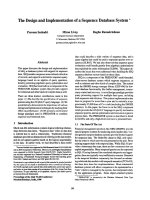
The equivalent channel is described in figure 1.
(13)
channel
w=U*w~CN(0,N01)
y
Figure 1. Equivalent channel of MIMO channel through SVD
n rair.
in for m a t ton /
stream«
Figure 2. Architecture of MIMO with SVD
Figure 2 shows the architecture for a MIM O communication system using SVD
with Waterfilling. The transmitter only allocates power to r eigen chan neh and no
power to other ones.
2.1.2 Rank and Condition number
This section will show what are the key factors contributing to the capacity of a
M1MO channel. It is simpler to focus on two separate low and high SNR regimes. At
low SNR, the pow er policy will allocate all power to the strongest eigenchannel. The
M IMO channel then provides only power gain:
C
P_
~Nn
(max X] )log2 e bits/s/Hz
/ '
(14)
It is more com plex situation at high SNR regime. At approximation level, the

capacity in (5) is restated as:
C
I log
/=1
k N a ,
k
k log SNR + log
i=i
bits/s/Hz (15)
where k is the number o f non-zero eigenvalues A 2, i.e rank o f H , and SNR = P/N„.
The parameter r is called num ber o f spatial degrees o f freedom pe r secon d per hertz
[8], It expresses the dimension of received signal through the M IMO channel, i.e.
dimension of signal H x This number depends strongly on H which describes the
transmission environment. Hence the MIMO channel with r non-zero eigenvalues
provides r degrees o f freedom.
Let us look at the capacity approximation at higher accuracy by using Jensen’s
inequality:
1 k
7 1 log
k /=!
1 +
p_
kN,'
A2
<
log
1 +
P
k N n
1 k

\\
(16)
In which
¿ / l ; = î ' ' [ h h ' ] = X K ,|2
/' = 1 /./
(17)
represents the total power transmitted. Equation ( 16) states that, for a given total
transmitted power, the capacity is maximized when all eigenchannels are equal, i.e
all eigenvalues are the same. It is clear that more subchannels convey a larger capacity
than fewer subchannels. In fact, however, this situation is rarely achieved since the
environment is not scattering rich enough.
2.2 Physical M IM O model
In this section, we will look into physical environmental factors contributing to
the M IM O channel performance in three main models: SIMO, M ISO and MIMO. We
also find the relationship between the key factors in the mathematical model and those
in the physical model in the case of MIMO channel. In addition, we only pay attention
to uniform antenna arrays in this section, that is, all antennas are aligned and equally
separated in the transmit and receive antenna arrays.
8
2.2.1 Line of sight SIMO
The model o f this case is shown in figure 3, in which there is no obstacle between
the transmitter and receiver, hence there is only direct path to the receiver. The antenna
separation is AtAc, in which Ac is the receive antenna separation normalized to the
carrier wavelength and Xc is the wavelength of the carrier.
The continuous-time impulse response /?,(t) between the transmit antenna and the /'
receive antenna is given as:
where a is the attenuation of the path, c is the speed o f light and dt is the distance from
the transmit antenna to the i[h receive antenna. The baseband channel gain with
assumption that d /c « M W (W is the bandwidth) is given as follows:
wheref c is the carrier frequency.

Let h be the channel matrix, h =[h, h2 hM]', then the SIMO channel can be
written as
where x is the transmitted symbol, n ~ C N (0, No I ) is the noise and y is the received
signal vector, h is sometimes called the signal direction or the spatia l signature [8]
caused by the transmitted signal on the receiver.
Because the distance between the transmitter and the receiver is much larger than
the antenna separation, d t can be approximated as:
hl (r) = ad( r - d r) i r 1.2
(18)
(19)
y - h*x + n
( 20)
dt » d + (/ - \)ArAc cos (j),
(21)
9
R \ anlcnna 1
(a)
Tx anlcnna k
(b)
Figure 3. Line of sight SÏMO and Line of sight M1SO channels
where d is the distance from the transmit antenna to the first receive antenna and (j) is
the angle of receive antenna array and the incident direction o f transmitted signal. The
second term on the right hand of (21) stands for the displacement of the receive
antenna i from antenna 1. The channel matrix is therefore given as:
h = a exp
v /
e x p ( - / 2 ,tA £2 )
exp(~y2/r(»,. - 1)A,Q)
( 22)
To get the maximum capacity, the receiver has to project the noisy signal onto the

signal direction using, e.g , maximal ratio combining (MRC) or receive beamforming
(RBF). The optimal capacity therefore is
C = log
g N
N n
,2 \
log
1 +
Peru,
bits/s/Hz
(23)
It is clear that the S1MO channel just gives the power gain M but no gain in the
degree of freedom.
2.2.2 Line of sight MISO
10
The model o f MISO line-of- sight is illustrated as in figure 3b which has N
transmit antennas and only 1 rcceive antenna. If <j) is the difference angle between the
transmit antenna array and the transmitted signal, and AtXc is the spacing between
antennas, then the M ISO channel is given as:
and Q = cos <f>.
The maximum capacity can be reached by performing beamforming algorithm
according to h. The capacity is as given in (23) in which the M ISO channel does not
supply any degree - o f - freedom gain.
2.2.3 Antenna arrays with only I.OS path
Does the M IM O channel provide degree - of - freedom with only direct path?
We are now considering the M IMO channel as in figure 4. In this model, let A, and Ar
be normalized transmit antenna spacing and receive antenna spacing, respectively. Let
hjk be the gain from kJh transmit antenna to ith receive antenna:
where d lk is the distance between the receive antenna i'h and the transmit antenna kth. If
the distance between two antenna arrays is much larger than the size o f each array, the

distance dlk can be approximated as follows:
here d is the distance from the transmit antenna I and the receive antenna 1. By
substituting (27) into (26) wc have:
y = h*x + /7
(24)
where
r
(25)
L
exp(- j2 n ( n r - ])Ar£2)J
hlk = a e x p ( - j27tdik / A )
(26)
d ik — d + (z - 1 )ArAc cos cj)r - (A - 1 )A, Ac cos <t>t
(27)
hlk = a exp - exp( /2^(A' - l)A,i2, )e xp (/2 ^(/ - l)A ,Q r ) (28)
V K
and the channel matrix can be written as:
(29)
where
ex p (- /2/rA,Q) exp(-/2;rA ,.Q )
(30)
exp(-y'27r(w, - l)A,Q)
x p ( - j 2 x ( n r - 1)A,Q)
and Q, = cos </>,. Q { - cos (/>,.
Since the propagation distance is much bigger than the antenna arrays’ size, the
capacity of this model is still as in (23) which states that antenna arrays with only LOS
path and arrays’s size being much smaller than the transmission distance does not
provide any degree o f freedom.
2.3 Key parameters in MIM O channel
In the cases above, it is clear that although there are multiple antennas at the

transmitter, at the receiver or at the both, we just obtain only the power gain which
increases the capacity logarithmically. This emerges a question that how to obtain
some degree - o f - freedom, hence linear gain in the capacity? And what is the
important factor to achieve this gain? This section will clarify which are the key
factors in the M IM O channel to achieve degree - o f - freedom gain.
Lets look at the primary formula for capacity o f the M IMO channel as in (2)
which would becom e (5) if the channel matrix H has more than 1 eigenvalue. We will
find out this condition in the physical model.
2.3.1 Antenna separation [4]
In this part we will study the effect o f antenna separation on the capacity of
M IMO channel. The channel model is as in figure 4 with assumption that there is only
LOS propagation. Let d { and d, be antenna spacing at Tx and Rx, respectively, which
are constant but can be adjustable. Tx antenna is placed in the jrz-plane with the lower
end at the origin and R is direct distance from the Tx origin to lower end o f Rx. In
addition, 6t, 0r, <p,. are angles in the local spherical coordinate system at the Tx and Rx.
Because we focus on antenna spacing, only LOS path is analyzed at this situation.
C = log: (dct(/ +H Hp))
(31)
Figure 4. A general MI1MO system with ULAs at both the Tx and Rx
Using ray-tracing method, the authors in |3| model the link as:
( x * \ ( - 2 n
i = e x P J — rm
V *
(32)
where rmn is path length from Tx antenna n lh to Rx antenna m lh, X is the wavelength.
According to [3], rmn can be approximated with the assumption that R is much larger
than antenna arrays’ size:
rmn = [(/? -I- m dr sin 0r cos (f>r - nd , sin 6, )2
+ (,m d, sin 0r sin <f>, )"
+ (,m d r cos 0' - nd, sin 0t )'

~ R + md,. sin 0r cos(f)r - nd t sin 0t
(m d r sin 6r sin <j)r )2 + (nu/r cos <9, - nd, cos 6*, )2
(33)
+ ■
2 R
(34)
For simplicity, we consider that Tx and Rx antenna arrays are parallel. The
receive vector from the /7th Tx antenna is:
exp
'0 .n
, ,exp
j2,T
I A
M-ljt
(35)
and the channel matrix is:
H los = [h(i, hi, , hN_i] (36)
The matrix H will have a high rank if its columns are uncorrelated, i.e.
13
/
(37)
(38)
(39)
From (38) we see that there are several solutions for high rank condition.
However we choose the one which has the shortest antenna spacing as in (39).
This product (d 4 r) is called Antenna Separation P roduct (ASP) [3] which is the key
design parameter. It is clear that ASP depends on the transmit-receive distance, the
wavelength, the num ber of antennas and 6r, 0,. A deviation factor is defined to test
how sensitive the performance is as the ratio o f the optimal ASP to current one
Figure 5 below shows the eigenvalues o f matrix H versus different values of r|

and figure 6 shows the capacity of a 3x3 MIMO channel for different values of rj. At
r)=0dB, i.e. A SP equals to A SPop[, three eigenvalues are the same which corresponds to
the m aximum capacity condition. Too large or too small antenna spacing results in
degradation in channel capacity.
Ergotiic capacity, C (bit/s/Hz)
14
Figure 5. Eigenvalues for 3x3 IMIMO system as a function of deviation factor in dB for
pure LOS channel
Figure 6. The capacity of MIMO system
15
2.3.2 Resolvability in the angular domain |X]
The separation in directional cosine does not ensure full-rank condition for the
channel matrix H. In fact, it can still be ill-conditioned if the angular condition is not
satisfied. In other words, the less aligned the spatial signatures are, the better the
condition o f H is. The angle # between two spatial signatures is:
| co s # | := |e r (Q ,.)* er (i2 J (41)
Define:
/ ,( £ ! ,, er ( n , ,) * e , ( n , - ) (42)
which just depends on Q, := £lr] - Q r2 By substituting (30) into (42) we get
/ r ( « r )
1 i a o ( in s i n ( / r Z . , )
— exp(//rA,i ! , ( //, -1 ))— 7 -7— v
nr s in (^ lri 2( / nr )
(43)
where Lr ni A, is the normalized antenna separation. Thus:
sin (nLr£l, )
co s#
7 , sin (/rZ,,fir / n, )
(44)
This parameter decides the condition of the matrix H. For simplicity, we suppose

that ai = a2 = a, then the eigenvalues o f H are:
A2 = a 2 /7 ,. (l +| costfj), A] = a 2n r (l-¡cos#|)
(45)
The matrix H will be ill-conditioned if |cos(0)| * I. Function /;.(.) as defined in
(43) has following properties:
• f r (Q, ) peaks at D, = 0 ; f(0 ) = 1;
• ) is periodic with period nr/L, = 1/ A,;
• f r ( Q ,) = 0 at Q r = k/Lr, k = 1,2, , nr — 1.
16
ç.
¿ n
Figure 7. f r\Q , ) plotted as a function of il, lor fixed Lr = 8 and different number of
receive antennas n,
Function /,(.) is plotted in figure 7 for different numbers of receive antennas nr.
To sum up, the angle resolution has to be large enough to ensure the matrix channel H
being well-conditioned for whatever the antenna separation is. It means that the
transmit-receive distance relative to the antenna arrays’ size will decide whether the
matrix H is well-conditioned or not.
2.4 Antenna Selection Algorithm
M IMO systems are not always well- conditioned and the channel matrix has low
rank, leading to key-hole or pin-hole phenomenon. In such situations, power will be
wasted if we use all analog chains in a M IMO system, especially in small
comm unication handsets whose power is limited. The author of this thesis and his
colleagues have proposed an antenna selection algorithm 17] to remove those inactive
antennas in rank-deficient indoor MIMO systems. We will numerically, using
simulation, demonstrate the correspondence between rank deficiency of an indoor
M IM O and the extent to which the number of receive antennas can be reduced
Rank-deficiency is related to the structure o f sca ttering in the propagation paths
and the classical single-scattering M IMO model cannot adequately explain this
phenomenon. Recently a double-scattering M IMO model (i.e. both transmit and

receive antenna arrays are obstructed by nearby scatterers), has been proposed in
which the channel matrix is characterized by a product o f two statistically independent
complex Gaussian matrices [15]. This double-scattering model can decouple (i.e. can
capture separately) the effects of rank-deficiency and spatial fading correlation in