ROBUST ADAPTIVE CONTROL OF MOBILE MANIPULATOR
Bạn đang xem bản rút gọn của tài liệu. Xem và tải ngay bản đầy đủ của tài liệu tại đây (3.27 MB, 32 trang )
TẠP CHÍ PHÁT TRIỂN KH&CN, TẬP 12, SỐ 16 - 2009
Bản quyền thuộc ĐHQG-HCM Trang 19
ROBUST ADAPTIVE CONTROL OF MOBILE MANIPULATOR
Tan Lam Chung
(1)
, Sang Bong Kim
(2)
(1) National Key Lab of Digital Control and System Engineering, VNU-HCM
(2) Pukyong National University, Korea
ABSTRACT: In this paper a robust control is applied to a two-wheeled mobile
manipulator (WMM) to observe the dynamic behavior of the total system. To do so, the
dynamic equation of the mobile manipulator is derived taking into account parametric
uncertainties, external disturbances, and the dynamic interactions between the mobile
platform and the manipulator; then, a robust controller is derived to compensate the
uncertainty and disturbances solely based on the desired trajectory and sensory data of the
joints and the mobile platform. Also, a combined system which composed of a computer and a
multi-dropped PIC-based controller is developed using USB-CAN communication to meet the
performance of demand of the whole system. What’s more, the simulation and experimental
results are included to illustrate the performance of the robust control strategy.
Keywords: robust adaptive controller, mobile manipulator
1. INTRODUCTION
The design of intelligent, autonomous machines to perform tasks that are dull, repetitive,
hazardous, or that require skill, strength, or dexterity beyond the capability of humans is the
ultimate goal of robotics research. Examples of such tasks include manufacturing, excavation,
construction, undersea, space, and planetary exploration, toxic waste cleanup, and robotic
assisted surgery. Robotics research is highly interdisciplinary requiring the integration of
control theory with mechanics, electronics, artificial intelligence, communication and sensor
technology.
A mobile manipulator is of a manipulator mounted on a moving platform. Such the
combined system has become an attraction of the researchers throughout the world. These
systems, in one sense, considered to be as human body, so they can be applicable in many
practical fields from industrial automation, public services to home entertainment.
In literature, a two-wheeled mobile robot has been much attracted attention because of its
usefulness in many applications that need the mobility. Fierro, 1995, developed a combined
kinematics and torque control law using backstepping approach and its asymptotic stability is
guaranteed by Lyapunov theory which can be applied to the three basic nonholonomic
navigations: trajectory tracking, path following and point stabilization [2]. Dong Kyoung
Chwa et al., 2002, proposed a sliding mode controller for trajectory tracking of nonholonomic
wheeled mobile robots presented in two-dimensional polar coordinates in the presence of the
external disturbances [5]; T. Fukao, 2000, proposed the integration of a kinematic adaptive
controller and a torque controller for the dynamic model of a nonholonomic mobile robot [4].
On the other hand, many of the fundamental theory problems in motion control of robot
manipulators were solved. At the early stage, the major position control technique is known to
be the computed torque control, or inverse dynamic control, which decouples each joint of the
robot and linearizes it based on the estimated robot dynamic models; therefore, the
performance of position control is mainly dependent upon the accurate estimations of robot
dynamics. Spong and Vidyasaga [8] (1989) designed a controller based on the computed
torque control for manipulators. The idea is to exactly compensate all of the coupling
Science & Technology Development, Vol 12, No.16 - 2009
Trang 20 Bản quyền thuộc ĐHQG-HCM
nonlinearities in the Lagrangian dynamics in the first stage so that the second stage
compensator can be designed based on linear and decoupling plant. Moreover, a number of
techniques may be used in the second stage, such as, the method of stable factorization was
applied to the robust feedback linearization problem [9] (1985). Corless and Leitmann [10]
(1981) proposed a theory based on Lyapunov’s second method to guaranty stability of
uncertain system that can apply to the manipulators.
In this paper, a robust control based on the work of [11] was applied to two-wheeled
mobile platform and a 6-dof manipulator taking into account parameter uncertainties and
external disturbances. In [11], the controller was only applied to a two-link manipulator, and
the platform is fixed. To design the tracking controller, the posture errors of the mobile
platform and of the joints are defined, and the Lyapunov functions are defined for the two such
subsystems and the whole system as well. The robust controllers are extracted from the
bounded conditions of the parameters, disturbances and the sensory data of the mobile
manipulator. Also, the simulation and experimental results show the effectiveness of the
system model and the designed controllers. And this works was done in CIMEC Lab.,
Pukyong National University, Pusan, Korea.
2. DYNAMIC MODEL OF THE WMM
The model of the mobile manipulator is shown in Fig. 1.
First, consider a two-wheeled mobile platform which can move forward, and spin about its
geometric center, as shown in Fig. 2. The length between the wheels of the mobile platform is
b2 and the radius of the wheels is
w
r . Y}{OX is the stationary coordinates system, or world
coordinates system; }{Pxy is the coordinates system fixed to the mobile robot, and
P
is placed
in the middle of the driving wheel axis; ),(
cc
yxC is the center of mass of the mobile platform
and placed in the x-axis at a distance d from
P
; the length of the mobile platform in the
direction perpendicular to the driving wheel axis is
a
and the width is
L
. It is assumed that the
center of mass C and the origin of stationary coordinate
P
are coincided. The balance of the
mobile platform is maintained by a small castor whose effect we shall ignore.
Fig 1. Model of the mobile manipulator
TẠP CHÍ PHÁT TRIỂN KH&CN, TẬP 12, SỐ 16 - 2009
Bản quyền thuộc ĐHQG-HCM Trang 21
2
r
w
x
p
b
X
Y
y
p
x
y
C
P
L
a
O
x
c
y
c
d
a=550
b=260
r
w
=220
L=400
d=0
Fig 2. Mobile platform configuration
Second, the manipulator used in this application is of an articulated-type manipulator with
two planar links in an elbow-like configuration: three rotational joints for three degrees of
freedom. They are controlled by dedicated DC motors. Each joint is referred as the waist,
shoulder and arm, respectively. Also, the manipulator has a 3-dof end-effector function as roll,
pitch and yaw; and a parallel gripper attached to the yaw.
The length and the center of mass of each link are presented
as ),(
11 bb
ZL , ),(
22 bb
ZL , ),(
33 bb
ZL , ),(
44 bb
ZL , ),(
55 bb
ZL , respectively. The geometric model
and the coordinate composed for each link is shown in Fig. 3.
105
-105
Z1
X0
105
-105
105
-15
X2
L
b1
=276
Z2
L
b2
=266
-105
105
-105
105
0
360
X3
Z3
L
b3
=256
L
b4
=150
L
b
5
=
1
4
0
X4
X5
X6
Y6
Z
b1
=138
Z
b2
=133
Z
b3
=128
1
2
3
4
5
6
Link 3
Arm
Link 2
Shoulder
Link 1
Waist
Pitch
Gripper
Roll
Yaw
Base
Z4
L
b
6
=
5
0
Y5
X7
Y7
Z7
X1
Z0
Y4
Y3
Z5
Z6
Fig 3. Geometry of 6-dof manipulator
Science & Technology Development, Vol 12, No.16 - 2009
Trang 22 Bản quyền thuộc ĐHQG-HCM
The dynamics of the mobile manipulator subject to kinematics constraints is given in the
following form [11]:
a
vv
d
d
v
T
v
a
v
a
v
E
qA
F
F
q
q
CC
CC
q
q
MM
MM
2
1
2
1
2221
1211
2221
1211
0
)(
(1)
The system constraint Eq. (1) can be simplified to the nonholonomic constraint of the
mobile platform only as follows:
0)(
vvv
qqA
(2)
where
rm
v
R
represents the actuated torque vector of the constrained coordinates;
)( rmmx
v
RE
, the input transformation matrix;
n
b
R
, the actuating torque vector of the free
coordinates;
1d
and
2d
, disturbance torques.
According to the standard matrix theory, there exists a full rank matrix
)(
)(
rmmx
vv
RqS
made up by a set of smooth and linearly independent vector spanning the
null space of
v
A , that is, 0)()(
v
T
vv
T
qAqS . From Eq. (2), we can find a velocity input vector
nm
Rt
)(
such that, for all t,
)(
vv
qSq
(3)
The Eq. (3) is called the steering system, and
is known as a velocity input to steer the state
vector
q
in state space. Furthermore, )(
v
qS is bounded by
sv
qS
)( ,
s
is a positive number.
2.1 Tracking Controller for the Mobile Platform
e
3
),,(
rrr
yx
r
),(
r
y
r
x
Reference trajectory
x
R
X
Y
e
1
e
2
x
r
y
y
r
x
y
P
Fig 4. Kinematic analysis of tracking problem
TẠP CHÍ PHÁT TRIỂN KH&CN, TẬP 12, SỐ 16 - 2009
Bản quyền thuộc ĐHQG-HCM Trang 23
The tracking errors of the mobile platform are given as follows [2]:
r
r
r
yy
xx
e
e
e
e
100
0cossin
0sincos
3
2
1
(4)
The first derivative of errors yields
r
r
r
ev
ev
v
e
e
e
e
e
3
3
1
2
3
2
1
sin
cos
.
10
0
1
(5)
The Lyapunov function is chosen as
2
32
2
2
10
cos1
2
1
2
1
k
e
eeV
(6)
The derivative of
0
V can be derived as
)(
sin
)cos(
22
2
3
310 rrr
vek
k
e
evveV
(7)
The velocity control law
d
achieves stable tracking of the mobile platform for the
kinematic model as
3322
113
sin
cos
ekevk
ekevv
rr
r
d
d
d
(8)
Where
21
,kk and
3
k are positive values.
The Eq. (7) becomes
3
2
2
3
2
110
sin e
k
k
ekV
(9)
Clearly 0
1
V
and the tracking errors
T
eeee
321
,, is bounded along the system’s solution.
It is also assumed that not only the velocity of 0
r
v is constant with the orientation
r
but
also the reference angular velocity
r
is bounded and have its bounded derivative for all
t
.
From Eqs. (5), (6) and (9), it is shown that e and e
are bounded, so that
1
V
, that is,
1
V
is
uniformly continuous. Since
1
V does not increase and converges to some constant value, by
Barbalat’s lemma, 0
1
V
as 0
t . As
t
, the limit of Eq. (9) becomes
2
33
2
121
0 ekekk (10)
Eq. (10) implies that
0
31
T
ee as
t
.
From Eq. (5), the derivative of error
3
e is given
r
e
3
(11)
Substituting
in Eq. (11) by the kinematics control input
d
in Eq. (8), the following result
is derived
33223
sin ekveke
r
(12)
Since 0
3
e as
t
, the limit of Eq. (12) yields
r
veke
223
(13)
Science & Technology Development, Vol 12, No.16 - 2009
Trang 24 Bản quyền thuộc ĐHQG-HCM
Since
3
2
ev
r
has the limit equal to zero when
t
, the derivative of this term can be
derived as follows:
2
2
23
2
)( evkev
dt
d
rr
(14)
Since Eq. (14) is bounded,
2
2
ev
r
is uniformly continous. From Barbalat’s lemma,
2
2
23
2
)( evkev
dt
d
rr
tends to zero. Therefore,
3
2
ev
r
tends to zero, and thus
2
ev
r
tends to zero.
Because the velocity of
r
v is constant, 0
2
e as
t
from Eq. (14). Hence, the equilibrium
point 0
e is uniformly asymptotically stable.
2.2 Lyapunov function for the mobile platform
Consider the first
m
-equation of Eq. (1) as follows:
vvd
T
vavav
EAFqCqCqMqM
1112111211
(15)
Multiplying both sides by
T
S and using Eq. (3) to eliminate the constraint force term λ, it
yields
vd
fCM
111111
(16)
Here SMSM
T
1111
, SMSSCSC
TT
111111
, )(
112121
FqCqMSf
aa
T
,
1
1
d
T
d
S
,
vv
T
v
ES
, and
ww
ww
v
T
rbrb
rr
ES
//
/1/1
It can be seen that
1
f , which consists of the gravitational and friction force vector
1
F and
the dynamics interaction with the manipulator )(
1212 aa
qCqM
, and the disturbances on the
mobile platform (terrain disturbance force) needs to be compensated online.
Property 1:
1111
2CM
is skew-symmetric
Property 2:
b
T
MSMSM
111111
and
b
MM
1212
Property 3: qCSCSC
b
T
111111
and qCC
b
1212
Assumption 1: Disturbance on the mobile platform is bounded, that is,
11 Nd
, with
1N
is
a positive constant.
Assumption 2: The friction and gravity on the mobile platform are bounded
by qqqF
vv
101
),(
, where
0
and
1
representing some positive constants.
The velocity tracking error is defined as
d
~
(17)
then, the mobile platform dynamics in terms of velocity tracking error is derived as
vddd
fCMCM
1111111111
~
~
(18)
Let us consider the following Lyapunov function
~~
2
1
111
MV
T
(19)
and the derivative of
1
V can be derived as follows:
TẠP CHÍ PHÁT TRIỂN KH&CN, TẬP 12, SỐ 16 - 2009
Bản quyền thuộc ĐHQG-HCM Trang 25
)(
~
1111111 dddv
T
fCMV
(20)
2.3 Lyapunov function of the manipulator
Consider the last n-equations of Eq. (1),
advvaa
FqCqMqCqM
2221212222
)(
(21)
Equation (21) represents the dynamic equation of the manipulator. In this equation, the
unknown terms need to be compensated are the gravitational and friction force
2
F , the
dynamic interaction term )(
2121 vv
qCqM
, and the disturbances on the manipulator.
Property 4:
2222
2CM
is skew-symmetric
Property 5:
b
MM
2121
and
b
MM
2222
Property 6: qCC
b
2222
and qCC
b
2121
Assumption 3: Disturbance on the manipulator is bounded, that is,
22 Nd
, with
2N
is
a positive constant.
Assumption 4: Friction and gravity in Eq. (21) are bounded by qqqF
322
),(
,
where
2
and
3
representing some positive constants.
The joint tracking error is defined, and its derivatives are derived as follows:
aada
aada
qqq
qqq
~
~
(22)
Also, the filter tracking error and its derivative,
)
~
(
~~
0,
~
~
aaaadaaa
T
aaa
qkrkqqqkqr
kkqkqr
(23)
The manipulator dynamics equation can be formulated in terms of filtered tracking error as
follows:
adaaa
fqkrCkMrM
22222222
)
~
)((
(24)
where )(
2212122222
FqCqMqCqMf
vvadad
The Lyapunov function for the manipulator is defined as
a
T
a
rMrV
222
2
1
(25)
the time derivative of
2
V can be derived as follows
]
~
)([
2
1
22222222
22222
daaa
T
a
a
T
aa
T
a
fkrMqkCkMr
rMrrMrV
(26)
2.4 Lyapunov function of the mobile manipulator
The Lyapunov function for the overall system, the mobile platform and the manipulator,
can be defined and rearrange as follows:
Science & Technology Development, Vol 12, No.16 - 2009
Trang 26 Bản quyền thuộc ĐHQG-HCM
)
~
(
2
1
)(
~~
2
1
2
1
)
~
(
~
)(
~
2
1
2
1
)
~
(
2
1
)
~
(
2
1
)
~
()
~
(
2
1
~
~
2
1
12210
2212110
2212110
221212110
2212
1211
0
SMrVVV
rMrSMrMV
rMrSMrSMSV
rMrrMSSMrSMSV
r
S
MM
MM
r
S
VV
TT
a
a
T
a
TT
a
T
a
T
a
TT
a
TT
a
T
aa
TTT
a
T
a
T
T
a
(27)
Taking the time derivative of V yields
)
~
(
21210
SMr
dt
d
VVVV
T
a
(28)
Substituting (20), (26) into (28) yields
)
~
(
~
)(
)(
~
2122222222
1111110
SMr
dt
d
fkrMqkCkMr
fCMVV
T
adaaa
T
a
dddv
T
][
(29)
On the other hand,
1
f can be rewritten in terms of error tracking filter
a
r as follows:
1121212
11212121212
11212
112121
)
~
)((
)()
~
)((
)
~
()
~
(
)(
fqkrkMCrMS
FqCqMSqkrkMCrMS
FqkrqCqkrkrqMS
FqCqMSf
aaa
T
adad
T
aaa
T
aaadaaaad
T
aa
T
(30)
with )(
112121
FqCqMSf
adad
T
Similarly,
2
f , in terms of velocity error
~
as follows:
2212121
2212121
222222121
2222221212
)
~
)(()
~
)((
)()(
)()(
)(
fSCSMSM
fSCSMSM
FqCqMSCSSM
FqCqMqCqMf
dd
adad
adadvv
(31)
with )(
222222
FqCqMf
adad
Substituting (30) and (31) into (29) yields
22110
~
~
d
T
aa
T
ad
T
v
T
rrVV
(32)
where
)
~
(
~
1212111111 aaa
T
dd
qkrkMqkCSfCM
dddaa
SCSMSMfqkkMCkrM
21212122222222
~
)(
The nonlinear terms
1
and
2
are need to be identical online using robust control scheme
in the following section based on the work in [14].
3. ROBUST CONTROLLER DESIGN
First, consider the second term of the Eq. (32) and using Properties (1)-(3) and
Assumptions (1)-(2):
TẠP CHÍ PHÁT TRIỂN KH&CN, TẬP 12, SỐ 16 - 2009
Bản quyền thuộc ĐHQG-HCM Trang 27
11
11012
111211
111211
1211
1112
111211
1121211111
~~
)(
~
)
~
(
~~
~
)
~
(
~~
~
)
~
(
~~
~
)
~
(
~
~
T
v
T
Nsaadbs
dbaaadbsdb
v
T
d
TT
aad
T
d
aaad
T
d
T
v
T
d
TT
aad
T
daaad
T
d
T
v
T
d
T
aaa
T
ddv
T
qqqkqC
qCqkrkqMM
SFSqkqCSC
qkrkqMSM
SFSqkqCS
CqkrkqMSM
qkrkMqkCSfCM
(33)
where the unknown vector
T
1
and the robust damping vector
1
are defined in the
following:
)1,,
~
,,)
~
(,(
)(,,,,,(
1
101121112111
qqqkqqqkrkq
CCMM
aaddaaadd
T
sNsbsbbsb
T
)
(34)
Second, consider the third term of the Eq. (32) and using Properties (4)-(6) and
Assumptions (3)-(4):
22
2322122
2122
222122
2122
222122
2122
2
2121
212222222
~
)
~
(
~
)
~
(
)
~
(
)()
~
(
~
)(
T
aa
T
a
Ndsbaadb
ddbaaadb
aa
T
a
ddaad
ddaaad
T
aa
T
a
ddaad
ddaaad
T
aa
T
a
d
T
a
dd
daaa
T
a
rr
qCqqkqC
SSMqkrkqM
rr
FSCqkqC
SSMqkrkqM
rr
FSCqkqC
SSMqkrkqM
rr
r
SCSM
SMfqkkMCkrM
r
q
(35)
where the unknown vector
T
2
and the RDC vector
2
are defined as follows:
)1,,,
~
,,)
~
((
,,,,,(
2
23122212222
qqqqkqSSqkrkq
CCMM
daadddaaad
T
sbbbb
T
)
N2
Let us choose the mobile platform and manipulator torque inputs as
2
111
~~
kk
pvv
(36)
2
222
aapaa
rkrk
(37)
Science & Technology Development, Vol 12, No.16 - 2009
Trang 28 Bản quyền thuộc ĐHQG-HCM
where ,0
pv
k 0
pa
k , 0
11
k ,and 0
22
k are the controller gains;
1
and
2
are the robust
damping control vectors, respectively. Then the tracking errors of the closed-loop system are
guaranteed to be globally uniformly ultimately bounded.
Substituting (36) and (37) into (32) yields
min
2
max
2
2
2
2
2
1
1
1min
2
2
2
1
2
1
2
2
2
22
2
1
1
110
2
2
2
2
2
2
2
22
2
1
2
1
2
1
1
110
2
22
2
2
2
2
1
11
2
1
2
10
22
2
2
2
211
2
1
2
10
22
2
2211
2
110
222
4422
4
2
4
2
~~~~~
kk
r
k
k
kkk
rk
k
kV
k
k
rk
k
k
kV
k
r
rk
k
kV
rrkkV
rrrkrrkkkVV
ad
ad
ad
a
a
d
d
aadd
T
aa
T
aa
T
apa
TTTT
pv
(38)
where
21min
,min kkk and
21max
,max
In Eq. (38),
max
is a bounded quantity; therefore, V decreases monotonically until the
solutions reach a compact set determined by the right-hand-side of Eq. (32). The size of the
residual set can be decreased by increasing
min
k . According to the standard Lyapunov theory
and the extension of the LaSalle theory, this demonstrates that the control input Eqs. (36) and
(37) can guarantee global uniform ultimate boundedness of all tracking errors.
Block diagram of robust controller is shown in Fig. 5
TẠP CHÍ PHÁT TRIỂN KH&CN, TẬP 12, SỐ 16 - 2009
Bản quyền thuộc ĐHQG-HCM Trang 29
Platform’s Robust Controller
Manipulator
Mobile
Platform
1
v
)E(
pv
k
Kinematics
Controller
Coord.
Tranform
Trajectory Planning
v
S
Filter Tracking Error
a
r
1
Eq. (2.39)
Motion Planning
Desired Trajectory
v
a
q
a
r
r
r
r
y
x
q
a
q
ad
q
a
q
~
a
r
dt
d
v
d
d
d
v
d
v
q
+
-
+
+
-
-
+
-
+
-
v
q
~
e
~
v
y
x
q
v
11
k
2
22
k
pa
k
Eq. (5.4)
Eq. (5.2)
a
r
Manipulator’s
Inverse kinematics
Cartesian
space
Joint
space
ad
q
ad
q
ad
q
ad
q
Eq. (2.32)
a
q
~
v
q
d
ad
q
ad
q
d
d
a
q
~
a
q
a
r
Manipulator’s Robust Controller
Eq. (2.28)
Fig 5. Block diagram of robust controller
4. CONTROL SYSTEM DEVELOPMENT
The control system is based on the integration of computer and PIC-based microprocessor.
The computer functions as high as high level control for image processing (not presented in
this paper) and control algorithm and the microprocessor, as low level controller for device
control. The configuration diagram of the overall control system is shown in Fig. 6. In the
configuration, there are 8 Servo-CAN modules are used to control all low-level devices: waist
motor, shoulder motor, arm motor, roll motor, pitch motor, and yaw motor for manipulator;
and left-wheeled and right-wheeled motors for mobile platform. The positions of the
manipulator’s joints feedback to the computer via ADC module on USB-CAN. The Servo-
CAN module is based on PIC18F458 shown in Fig. 8. The USB-CAN module is used to
interface between high and low levels: it transforms the serial data from computer to CAN
messages shown in Fig. 7. The USB-CAN interface is shown in Fig. 9.
For the operation, USB camera Logitech 4000 is used to capture the image stream into
memory with size of 320x240 at 30fps using QuickCam SDK. The image is processed using
image processing library OpenCV to extract the features from the image for the object’s
position detection. The torque command is sent to the low level to control the mobile platform
and the manipulator to perform a certain task. The total control processes are programmed and
Science & Technology Development, Vol 12, No.16 - 2009
Trang 30 Bản quyền thuộc ĐHQG-HCM
integrated into the interface IMR V.1 in Visual C++ shown in Fig. 10. With this interface, the
mobile manipulator’s parameters can be set before the operation.
FT245BM
USB Controller
PIC18F458
USB/CAN Controller
TX-CAN RX-CAN
MCP2551
CAN Transceiver
93C64
EEPROM
Parallel Comm.
USB Comm.(12Mbs)
(1Mbps)
CAN Network
USB-CAN
Module
Computer
P4-2.8
PIC18F458
Servo CAN
PIC18F458
Servo CAN
PIC18F458
Servo CAN
PIC18F458
Servo CAN
PIC18F458
Servo CAN
PIC18F458
Servo CAN
PIC18F458
Servo CAN
PIC18F458
Servo CAN
USB Camera
Logitech 4000
Left wheel
Right wheel
Pot.2
Pot.1
Pot.3
Pot.4
Pot.5
Pot.6
Waist motor
Shoulder motor
Arm motor
Roll motor
Pitch motor
Yaw motor
CAN comm. (1Mbps)
Enc.
Enc.
Enc.
Enc.
Enc.
Enc.
ADC
Module
Fig 6. Diagram of the control system
TẠP CHÍ PHÁT TRIỂN KH&CN, TẬP 12, SỐ 16 - 2009
Bản quyền thuộc ĐHQG-HCM Trang 31
Fig 7. USB-CAN module
Fig 8. Servo CAN module
Science & Technology Development, Vol 12, No.16 - 2009
Trang 32 Bản quyền thuộc ĐHQG-HCM
Fig 9. USB-CAN Interface
Fig 10. Mobile manipulator interface IMR V.1
TẠP CHÍ PHÁT TRIỂN KH&CN, TẬP 12, SỐ 16 - 2009
Bản quyền thuộc ĐHQG-HCM Trang 33
5. SIMULATION RESULTS
To verify the effectiveness of the controller, the simulations have been done with
controller (8),(36) and (37) using Visual C++6 (with matrix package) and Gnuplot 4. The
reference trajectory are planned for the total system: a cubic spline reference line for the
mobile platform shown in Fig. 11 with the trajectory parameters in Fig. 12 and sinusoid
trajectory for joint 1 to joint 6 with the frequency of fffff 2.1,1.1,,9.0,8.0 and
f3.1 ( Hzf 3125.0 ) as shown in Fig. 21, respectively. The kinematic controller constants are
20,51
2
kk and 10
3
k . The robust controller gains
are 2.1,300,001.0,40
2211
kkkk
papv
. The mobile robot for the simulation has the
following parameters: mmb 200 , mmr 110
, kgm
c
6.20 , kgm
w
2.1 . The initial posture of
the mobile manipulator and the reference trajectory
is mx 1.0)0( , my 3.0)0( ,
45)0(
, mx
r
3.0)0( , my
r
5.0)0( , 0)0(
r
, respectively; the
initial joint positions, )6/,10/,18/,18/,10/,6/()0(
a
q .Sampling time is 10ms. The
disturbance is a random noise with the magnitude of 3, but it is not considered in this
simulation.
Simulation results are given through Figs. 13-29. The mobile platform‘s tracking errors are
given in Fig. 13 for full time (8s) and Fig. 12 for the initial time (2s), respectively. It can be
seen that the platform errors go to zero after about 1 second. The kinematics control input, the
linear and angular velocities at mobile platform center, is shown in Fig. 15; the velocities of
the left and right wheel, in Fig. 16. It can be seen that the tracking velocity is in the vicinity of
2m/s as desired, but it should be tuned for the acceptable value in the practical applications.
The robust vector for the mobile platform )6 1(
1
i
in the controller Eq. (36) is given in Fig.
17, and the torque on the left and the right wheel, in Fig, 18. The mobile platform’s tracking
position with respect to the reference trajectory is shown in Fig. 19 for the initial time (2s) and
in Fig. 20 for full time (8s). As for the manipulator, the tracking positions of joint 1 to joint 6
are shown in Figs. 22-27. It can be seen that the overall tracking performance is acceptable,
but they each are depend on the frequency of the reference trajectory. The joint’s position
errors and joint’s torques are shown in Figs. 28 and 29, respectively.
The experimental results are given through Figs. 30-39. The reference trajectory for the
experiment is designed again to be satisfied the mechanical condition of the experimental
mobile manipulator. The reference trajectory of the platform is given in Fig. 30. The posture of
the mobile platform can be calculated using dead-reckoning method via encoders, then the
errors
21
,ee and
3
e can be derived shown in Figs. 31- 33. The errors go to zero after about 3
seconds. The joint’s reference trajectory for the manipulator is designed as sinusoidal
trajectory with slower frequencies than those in the simulation, that is,
fffff 2.1,1.1,,9.0,8.0 and f3.1 ( Hzf 25.0 ). The joint’s position errors are shown in Figs. 34-
39, respectively; they are satisfied the tracking performance in the manner of ordinary
applications.
Overall, the simulation and experimental results are reasonably same; it can be concluded
that the kinematics controller and the robust controller are all applicable for practical fields.
The experimental test bed is shown in Fig. 40.
Science & Technology Development, Vol 12, No.16 - 2009
Trang 34 Bản quyền thuộc ĐHQG-HCM
0
500
1000
1500
2000
2500
3000
3500
4000
0 1000 2000 3000 4000 5000 6000 7000
Interpolated trajectory
Knot
X Coordinate (mm)
Y Coordinate (mm)
Fig 11. Cubic spline reference trajectory for platform
-5
-4
-3
-2
-1
0
1
2
3
0 1 2 3 4 5 6 7 8
Time (s)
Trajectory Parameter
Ref. linear velocity (m/s)
Ref. angular velocity (rad/s)
Ref. heading angle (rad)
Fig 12. Reference trajectory parameters for platform
TẠP CHÍ PHÁT TRIỂN KH&CN, TẬP 12, SỐ 16 - 2009
Bản quyền thuộc ĐHQG-HCM Trang 35
-800
-600
-400
-200
0
200
400
e
1
(mm)
e
2
(mm)
e
3
(rad);(1:1000)
0 1 2 3 4 5 6 7 8
Time (s)
Error e
i
Fig 13. Platform tracking errors for full time
-800
-600
-400
-200
0
200
400
0 500 1000 1500 2000
e
1
(mm)
e
2
(mm)
e
3
(rad);(1:1000)
Time (s)
Error e
i
Fig 14. Platform tracking errors for the initial time
Science & Technology Development, Vol 12, No.16 - 2009
Trang 36 Bản quyền thuộc ĐHQG-HCM
-15
-10
-5
0
5
10
0 1 2 3 4 5 6 7 8
Linear velocity (m/s)
Angular velocity (rad/s)
Time (s)
Velocity of center
Fig 15. Velocities of platform’s center
-400
-200
0
200
400
0 1 2 3 4 5 6 7
8
Time (s)
Angular velocity (rpm)
Left wheel velocity
Right wheel velocity
Fig 16. Wheel velocities
TẠP CHÍ PHÁT TRIỂN KH&CN, TẬP 12, SỐ 16 - 2009
Bản quyền thuộc ĐHQG-HCM Trang 37
-10
0
10
20
30
40
0 1 2 3 4 5 6 7 8
Time (s)
11
12
13
14
15
Robust vector
Fig 17. Robust vector of mobile platform
-15
-10
-5
0
5
10
15
0 1 2 3 4 5 6 7 8
Right torque
Left torque
Time (s)
Wheel torque (Nm)
Fig 18. Wheel’s torques of mobile platform
Science & Technology Development, Vol 12, No.16 - 2009
Trang 38 Bản quyền thuộc ĐHQG-HCM
0
200
400
600
800
1000
0 500 1000 1500 2000
X-coordinate (mm)
Y-coordinate (mm)
Mobile platform trajectory
Reference trajectory
Fig 19. Tracking trajectory of mobile platform (2s)
0
500
1000
1500
2000
2500
3000
3500
4000
0 1000 2000 3000 4000 5000 6000 7000 8000
Mobile platform trajectory
Reference
trajectory
X-coordinate (mm)
Y-coordinate (mm)
Fig 20. Tracking trajectory of mobile platform (8s)
TẠP CHÍ PHÁT TRIỂN KH&CN, TẬP 12, SỐ 16 - 2009
Bản quyền thuộc ĐHQG-HCM Trang 39
-1.0
-0.5
0
0.5
1.0
0 1 2 3 4 5 6 7 8
q
a1d
q
a2d
q
a3d
q
a4d
q
a5d
q
a6d
Time (s)
Desired joint coordinate (rad)
Fig 21. Joint reference trajectory
-0.8
-0.6
-0.4
-0.2
0
0.2
0.4
0.6
0.8
1.0
0 1 2 3 4 5 6 7 8
q
ad2
q
a2
Time (s)
Joint 1 coordinate (rad)
Fig 22. Tracking position of joint 1
Science & Technology Development, Vol 12, No.16 - 2009
Trang 40 Bản quyền thuộc ĐHQG-HCM
-0.8
-0.6
-0.4
-0.2
0
0.2
0.4
0.6
0.8
1.0
0 1 2 3 4 5 6 7 8
Time (s)
Joint 1 coordinate (rad)
q
ad1
q
a1
Fig 23. Tracking position of joint 2
-0.8
-0.6
-0.4
-0.2
0
0.2
0.4
0.6
0.8
1.0
0 1 2 3 4 5 6 7 8
Time (s)
Joint 3 coordinate (rad)
q
ad3
q
a3
Fig 24. Tracking position of joint 3
TẠP CHÍ PHÁT TRIỂN KH&CN, TẬP 12, SỐ 16 - 2009
Bản quyền thuộc ĐHQG-HCM Trang 41
-1.0
-0.8
-0.6
-0.4
-0.2
0
0.2
0.4
0.6
0.8
0 1 2 3 4 5 6 7 8
q
a4
q
a4d
Time (s)
Joint 4 coordinate (rad)
Fig 25. Tracking position of joint 4
-1.0
-0.8
-0.6
-0.4
-0.2
0
0.2
0.4
0.6
0.8
0 1 2 3 4 5 6 7 8
q
a5
q
a5d
Time (s)
Joint 5 coordinate (rad)
Fig 26. Tracking position of joint 5
Science & Technology Development, Vol 12, No.16 - 2009
Trang 42 Bản quyền thuộc ĐHQG-HCM
Time (s)
-1.0
-0.8
-0.6
-0.4
-0.2
0
0.2
0.4
0.6
0.8
0 1 2 3 4 5 6 7 8
Joint 6 coordinate (rad)
q
a6
q
a6d
Fig 27. Tracking position of joint 6
-0.6
-0.4
-0.2
0
0.2
0.4
0.6
0 1 2 3 4 5 6 7 8
q
a1e
q
a2e
q
a3e
q
a4e
q
a5e
q
a6e
Time (s)
Joint error (rad)
Fig 28. Joint position error
TẠP CHÍ PHÁT TRIỂN KH&CN, TẬP 12, SỐ 16 - 2009
Bản quyền thuộc ĐHQG-HCM Trang 43
-20
-10
0
10
20
0 1 2 3 4 5 6 7 8
T
a1
T
a2
T
a3
T
a4
T
a5
T
a6
Time (s)
Joint torque (Nm)
Fig 29. Joint torque
0.4
0.6
0.8
1.0
1.2
1.4
1.6
1.8
2.0
0.2 0.4 0.6 0.8 1.0 1.2 1.4 1.6 1.8
x Coordinate (m)
Y Coordinate (m)
(0.3,0.5) (0.5,0.5) (0.8,0.5)
(0.94,0.56)
(1.0,0.7)
(1.0,1.2)
(1.0,1.7)
(1.04,1.8)
(1.15,1.85)
(1.65,1.85)
Fig 30. Reference trajectory for the experiment