Analysis the Statistical Parameters of the Wavelet Coefficients for Image Denoising
Bạn đang xem bản rút gọn của tài liệu. Xem và tải ngay bản đầy đủ của tài liệu tại đây (516.92 KB, 7 trang )
VNU Journal of Natural Sciences and Technology, Vol. 29, No. 3 (2013) 1-7
1
Analysis the Statistical Parameters of the Wavelet Coefficients
for Image Denoising
Nguyễn Vĩnh An*
PetroVietnam University, 173 Trung Kính, Cầu Giấy, Hanoi, Vietnam
Received 14 September 2012
Revised 28 September 2012; accepted 28 June 2013
Abstract: Image denoising is aimed at the removal of noise which may corrupt an image during
its acquisition or transmission. De-noising of the corrupted image by Gaussian noise using wavelet
transform is very effective way because of its ability to capture the energy of a signal in few larger
values. This paper proposes a threshold selection method for image de-noising based on the
statistical parameters which depended on sub-band data. The threshold value is computed based on
the number of coefficients in each scale j of wavelet decomposition and the noise variance in
various sub-band. Experimental results in PSNR on several test images are compared for different
de-noise techniques.
1. Introduction
∗
∗∗
∗
Image de-noising is a common procedure in
digital image processing aiming at the removal
of noise which may corrupt an image during its
acquisition or transmission while sustaining its
quality. Noise is unwanted signal that interferes
with the original signal and degrades the quality
of the digital image. Different types of images
inherit different types of noise and different
noise models are used for different noise types.
Noise is present in image either in additive
or multiplicative form [1]. Various types of
noise have their own characteristics and are
inherent in images in different ways. Gaussian
noise is evenly distributed over the signal. Salt
and pepper noise is an impulse type of noise
_______
∗
Tel: 84-913508067.
E-mail:
(intensity spikes). Speckle noise is
multiplicative noise which occurs in almost all
coherent systems. Image de-noising is still a
challenging problem for researchers as which
causes blurring and introduces artifacts. De-noising
method tends to be problem specific and depends
upon the type of image and noise model.
De-noising based on transform domain
filtering and wavelet can be subdivided into
data adaptive and non-adaptive filters [2].
Image de-noising based on spatial domain
filtering is classified into linear filters and non-
linear filters [3, 4]. In [5, 6], the paper proposes
an adaptive, data driven threshold for image
denoising via wavelet soft thresholding.
A proposal of vector/matrix extension of
denoising algorithm developed for grayscale
images, in order to efficiently process
N.V. An / VNU Journal of Natural Sciences and Technology, Vol. 29, No. 3 (2013) 1-7
2
multichannel is presented in [7]. In [8], authors
propose several methods of noise removal from
degraded images with Gaussian noise by using
adaptive wavelet threshold (Bayes Shrink,
Modified Bayes Shrink and Normal Shrink).
This paper is organized as follows: A brief
review of DWT and wavelet filter banks are
provided in session II. In session III, the
wavelet based thresholding technique is
explained. The methods of selection of wavelet
thresholding is presented in IV. In session V the
new proposed thresholding technique for
denoising is presented. The experiment results
of this work are compared with others in
session VI and concluding remarks are given.
2. Discrete wavelet transform (DWT)
The mathematical approach of the discrete
wavelet transform (DWT) is based on
( ) ( )
k k
k
f t a t
ψ
=
∑
(1)
Where
k
a
are the analysis coefficients and
( )
k
t
ψ
is the analyzing functions, which are
called basic functions. If the basic functions are
orthogonal, that is
( ), ( ) ( ) ( ) 0
k l k l
t t t t dt
for k l
ψ ψ ψ ψ
= =
≠
∫
(2)
The coefficients can be estimated from the
following equation:
( ), ( ) ( ) ( )
k k k
a f t t f t t dt
ψ ψ
= =
∫
(3)
Wavelets consist of the dilations and
translations of a single valued function
(analyzing wavelet or basic wavelet or also
known as the mother wavelet)
2
( )
L R
ψ
∈
. The
family of function
,
s
τ
ψ
by dilations and
translations of
ψ
1/2
,
( ) , , 0
s
t
t s s R s
s
τ
τ
ψ ψ τ
−
−
= ∈ >
(4)
In general, a 2-D signal may be transformed
by DWT as
, ,
( ) ( )
j k j k
k j
f t a t
ψ
=
∑∑
(5)
Where
,
j k
a
and
,
( )
j k
t
ψ
are the transformed
coefficients and basis functions respectively.
Another consideration of the wavelets is the
sub-band coding theory or multi-resolution
analysis. The signal passes successively
through pairs of lowpass and high pass filters,
which produce the transformed coefficients
(analysis filters). By passing these coefficients
successively through synthesis filters, we
reproduce the original signal at the decoder. An
input signal S maybe equivalently analysed as:
3 3 2 1
S A D D D
= + + +
Level 3 (6)
2 2 1
S A D D
= + +
Level 2 (7)
1 1
S A D
= +
Level 1 (8)
Similarly, by using wavelet packet
decomposition, the signal may be analysed as
1 3 3 3 3
S A AAD DAD ADD DDD
= + + + +
(9)
The process of decomposition and
reconstruction is in figure 1.
N.V. An / VNU Journal of Natural Sciences and Technology, Vol. 29, No. 3 (2013) 1-7
3
S ig n a l
A 1 D 1
A 2 D 2
A 3 D 3
Fig. 1. Wavelet decomposition and reconstruction.
3. Wavelet thresholding
Let
{
}
, , 1, 2,
ij
f f i j M
= =
(10)
denote the M × M matrix of the original
image to be recovered and M is some integer
power of 2. Assume the signal function f is
corrupted by independent and identically
distributed (i.i.d) zero mean, white Gaussian
noise
ij
n
with standard deviation ơ i.e,
ij
n
~
N(0,
2
σ
), so that the noisy image is obtained.
ij ij ij
g f n
σ
= +
(11)
The goal is to estimate an
ij
f
∧
from noisy
ij
g
(M, N are width and height of image) such that
Mean Squared Error (MSE) is calculated in (12)
2
1 1
1
M N
ij ij
j i
MSE f f
MN
∧
= =
= −
∑∑
(12)
The observation model is expressed as
follows:
Y = X + V (13)
Here Y is wavelet transform of the noisy
degraded image, X is wavelet transform of the
original image and V denotes the wavelet
transform of the noise components in Gaussian
distribution
2
(0, )
v
N
σ
. Since X and V are
mutually independent, we have
2 2 2
y x v
σ σ σ
= +
(14)
It has been shown that the noise standard
deviation
2
v
σ
can be estimated from the first
decomposition level diagonal subband
1
HH
by
the robust and accurate median estimator [5].
( )
2
1
2
0.6745
v
median HH
σ
=
(15)
The variance of the sub-band of noisy
image can be estimated as (
m
A
are wavelet
coefficients of subband under consideration. M
is the total number of wavelet coefficient in that
sub-band)
2 2
1
1
M
y m
m
A
M
σ
=
=
∑
(16)
In figure 1 shown wavelet decomposition in
3 levels. The su-bands
, ,
k k k
HH HL LH
are
called the details (k is level ranging from 1 to
the largest number J). The
J
LL
is the low
resolution residue. The size of the subband at
scale k is
2 2
k k
M M
×
.
Fig.2. Sub-bands of the 2-D orthogonal wavelet
transform with 3 decomposition levels (H- High
frequency bands and L-Low frequency bands).
The wavelet threshold denoising method
filters each coefficient from the detail subbands
with a threshold function to obtain modified
coefficients. Threshold plays an important role
in the denoising process. There are two
thresholding methods in used. The hard
thresholding operator is defined as
N.V. An / VNU Journal of Natural Sciences and Technology, Vol. 29, No. 3 (2013) 1-7
4
D(U,λ) = U for all
U
> λ and D(U,λ) = 0
otherwise (17)
The soft thresholding operator on the other
hand is defined as
( , ) sgn( ) *max(0, )
D U U U
λ λ
= −
(18)
Hard thresholding is “keep or kill”
procedure and it introduces artifacts in the
recover images. Soft thresholding is more
efficient and it is used to achieved near minmax
rate and to yield visually more pleasing images.
The soft-threshold function (shrinkage
function) and the hard threshold as depicted in
figure 3.
(a) (b)
Fig. 3. Thresholding function (a) Soft threshold
(b) Hard threshold.
4. Methods of threshold selection for image
denoising
4.1. Universal threshold
Universal threshold can be defined as
2log( )
T N
σ
= (19)
N being the signal length i.e the size of the
image, ơ is noise variance.
This is easy to implement but provide a
threshold level much depend on the size N of
image resulting in smoother reconstructed
image. This threshold estimation does not care
of the content of the data and provide the value
larger than other.
4.2. Visu Shrink
Visu Shrink was introduce by Donoho [6].
It uses a threshold value that is proportional to
the standard deviation of the noise. The
estimation of ơ was defined by
(
)
1
1,
: 0,1, 2 1
0.6745
j
j k
median g k
σ
−
−
= −
=
(20)
Where
1,
j k
g
−
corresponds to the details
coefficients in the DWT. Visu Shrink does not
deal with minimizing the mean squared error
and can not remove speckle noise. It can only
deal with an additive noise and follow the
global threshold scheme. Visu shrink has a
limitation of not dealing with minimizing the
mean squared error, i.e it removes overly smoothed.
4.3. Sure Shrink
In Sure Shrink, a threshold is choosen based
on Stein’s Unbiased Risk Estimator(SURE) by
Donoho and Johnstone. It is a combination of
the universal threshold and SURE threshold [7]
so to be smoothness adaptive. This method
specifies a threshold value t
j
for each resolution
level j in the DWT. The goal of SURE is to
minimize the MSE, the threshold T is defined as
(
)
min , 2log
T t N
σ
=
(21)
Where t denotes the value that minimizes
SURE, ơ is the noise variance and N is the size
of the image. This method threshold the
empirical wavelet coefficients in groups rather
than individually, making simultaneous
decisions to retain or to discard all the
coefficients within non-overlapping blocks.
4.4. Bayes Shrink (BS)
Bayes Shrink was proposed by Chang, Yu
and Vetterli. The Bayes threshold T
B
is defined as
N.V. An / VNU Journal of Natural Sciences and Technology, Vol. 29, No. 3 (2013) 1-7
5
2
v
BS
x
T
σ
σ
=
(22)
Where
(
)
2 2
max
x y v
σ σ σ
= −
(23)
2
v
σ
is the noise variance which is estimated
from the sub-band HH and
y
σ
is the variance of
the original image. Note that in the case where
2 2 2
,
v y x
σ σ σ
≥
is taken to be zero. In practice,
we can choose
{
}
max
BS m
T A
=
and all
coefficients are set to zero.
Noise is not being sufficiently removed in
an image using Bayes Shrink method. So the
paper [8] referred to Modified Bayes Shrink
(MBS). It performs the threshold values that are
different for coefficients in each sub-band. The
threshold T can be determined as follows:
2
v
MBS
x
T
βσ
σ
=
(24)
where
log
2
N
j
β
=
×
(25)
N
is the total of coefficients of wavelet,
j
is the wavelet decomposition level present in
the sub-band under scrutiny.
4.5. Normal Shrink
The threshold value which is adaptive to
different sub-band characteristics
2
v
N
y
T
βσ
σ
=
(26)
Where the scale parameter β has computed
once for each scale using the following (27):
log
K
L
J
β
=
(27)
k
L
means the length of the sub-band at
th
k
scale.
J
is the total number of
decomposition. Where
2
v
σ
is the noise variance
which is estimated from the equation (15) and
y
σ
is the variance of the noisy image which is
calculated by equation (16).
5. The new proposal method
In Modified Bayes Shrink, the value of β in
equation (25) only count for N is the total of
coefficients of wavelet. So that the value of β is
something “globally”, which does not count for
the length of the sub-band at k
th
scale. We
present a new proposal function for threshold
T
N
MBS in equation (24)
2
v
MBS
x
T
βσ
σ
=
In our proposed method, the value of β is
substituted by
log
2
2
k
N
N
k
β
=
×
(28)
Here N/2
k
is the length of the sub-band at
scale k.
The image denoising algorithms that use the
wavelet transform consist of the following
steps:
1- Calculate the multiscale decomposition
wavelet transform of the noisy image.
2- Estimate the noise variance
2
v
σ
from the sub-
band
k
HH
and
x
σ
is variance of the original
image.
3- For each level k, compute length N of the
data.
4- Compute threshold based on equation (24)
and (28)
N.V. An / VNU Journal of Natural Sciences and Technology, Vol. 29, No. 3 (2013) 1-7
6
5- Apply soft threshold to the noisy coefficients.
6-Meger low frequency coefficients with
denoise high frequency coefficients in step 5.
7- Invert the wavelet transform to reconstruct
the denoised image.
8- Difference of noisy image and original image
is calculated using imsubract command.
9- Size of the matrix obtains in step 8 is
calculated
10- Each of the pixels in the matrix obtained in
the steps 8 is squared and calculate sum of all
the pixels.
11- MSE is obtained by taking the ratio of value
obtained in step 10 to the value obtained in the
step 9 as in equation (12).
12- PSNRis calculated by dividing 255 with
MSE, taking log base 10 as in (29)
The performance of noise reduction
algorithm is measure using Peak Signal to
Noise Ratio (PSNR) which is defined as
2
10
255
10log
PSNR dB
MSE
=
(29)
6. Experimental results and discussions
We try to compare above algorithm on
several test gray image like image of Lena and
image of House at Gaussian noise level with
noise standard deviation ơ = 0.01 and ơ = 0.04
using Daubechies wavelet with 3 level
decomposition.
Original Lena (Left) and noisy Lena with ơ = 0.01(Middle) and with ơ = 0.04 (Right)
Original House (Left) and noisy house with ơ = 0.01 (Middle) and ơ = 0.04 (Right)
Fig. 4. Images of Lena and House using for testing of denoising methods.
The original image and noised images of
Lena and House is in figure 4. Performance of
noise reduction is measured using Peak Signal
to Noise Ratio (PSNR) as in table 1.
From table 1, by using equation (24) and
(28) we calculated the values of PSNR for Lena
image and House image. The results by our
proposal method is significantly improved than
by using other method in term of denoising
images those are corrupted by Gaussian noise
during transmission which is normally random
in nature.
N.V. An / VNU Journal of Natural Sciences and Technology, Vol. 29, No. 3 (2013) 1-7
7
Tabel 1. Comparision of PSNR of different wavelet thresholding selection for images corrupted
by Gaussian noise
Image Noise
level
Universal
threshold
Visu
shrink
Bayes
shrink
Modified
Bayes shrink
Normal
shrink
Proposed
method
Lena 0.001 69.06 73.21 74.11 75.87 75.34 76.24
0.004 56.23 59.12 61.67 62.07 61.55 62.77
House 0.001 69.02 73.56 74.38 75.89 75.23 76.04
0.004 55.27 59.67 61.22 62.13 61.78 62.45
The proposed threshold estimation is based
on the adaptation of the statistical parameters of
the sub-band coefficients. Since the value of
proposed threshold is calculated dependent on
decomposition level with sub-band variance
estimation, the method yields significantly
superior quality and better PSNR.
References
[1] Matlab6.1 -Image Processing Toolbox‖,
http:/www.mathworks.com/access/helpdesk/hel
p/toolbox/images/
[2] Motwani, M.C., Gadiya, M.C., Motwani, R.C.,
Harris, F.C Jr. “Survey of Image Denoising
Techniques”.
[3] Windyga, S. P. 2001, “Fast Impulsive Noise
Removal”, IEEE transactions on image
processing, vol. 10, No. 1, pp. 173-178.
[4] Kailath, T. 1976, Equations of Wiener-Hopf
type in filtering theory and related applications,
in Norbert Wiener: Collected Works vol. III,
P.Masani, Ed. Cambridge, MA: MIT Press, pp.
63–94.
[5] S.Grace Chang, Bin Yu and M.Vattereli,
“Adaptive Wavelet Thresholding for Image
Denoising and Compression”, IEEE Trans
Image Processing, vol.9,pp.1532-1546, Sept
2000.
[6] D.L Donoho and I.M Johnstone, “Denoising by
soft thresholding”, IEEE Trans on Inform
Theory, vol 41, pp 613-627, 1995.
[7] F.Luisier, T. Blu and M. Unser, “A new SURE
approach to image denoising: Inter-scale
orthonormal wavelet thresholding”, IEEE
Trans. Image Processing, vol 16, no.3, pp.593-
606, Mar 2007.
[8] Iman Elyasi and Sadegh Zarmehi, “Elimination
Noise by Adaptive Wavelet Threshold”, World
Academy of Science, Engineering and
Technology 32, 2009.
Phân tích các tham số thống kê của các hệ số wavelet
dùng cho tách nhiễu ảnh
Nguyễn Vĩnh An
Trường Đại học Dầu khí Việt Nam, 173 Trung Kính, Cầu Giấy, Hà Nội, Việt Nam
Tóm tắt: Tách nhiễu cho ảnh nhằm mục đích khôi phục lại ảnh bị giảm chất lượng khi thu nhận và
trong quá trình truyền. Dùng biến đổi wavelet để thực hiện việc tách nhiễu Gaussian là rất hiệu quả do
hầu hết năng lượng của tín hiệu được dồn tập trung vào một số ít các hệ số. Trong bài báo này, tác giả
sẽ đề xuất một phương pháp lựa chọn mức ngưỡng trong quá trình tách nhiễu cho ảnh dựa vào các
tham số thống kê dữ liệu trong các dải băng con. Giá trị ngưỡng được tính toán căn cứ vào số các hệ
số trong mỗi mức phân tích j của phép phân tích wavelet và phương sai của nhiễu trong các dải băng
con khác nhau. Cuối cùng tác giả sẽ sẽ tiến hành so sánh hiệu quả của các phương pháp bằng thực
nghiệm dựa vào tỷ số tín hiệu trên nhiễu PSNR của một số bức ảnh có nội dung khác nhau để đánh giá
hiệu quả tách nhiễu.