Tài liệu Slide bài giảng môn Lý thuyết xác suất thống kê bằng Tiếng Anh StatisticsLecture3_Estimation

Parameter estimation
Parameter estimation


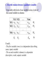
“ Estimation“: Using low accurate measuring tools (using data collected in a very limited sample of population) to determine as precisely as possible
value of a certain parameter (of all population).


An opinion or judgment of the worth,
extent, or quantity of anything, formed
without using precise data; as,
estimations of distance, magnitude,
mount, or moral qualities.




Parameter Estimation
Parameter Estimation
* Estimation methods
* Distribution of estimated parameters
* Comparing distribution of estimated
parameter wit Normal distribution
* Confidence Interval of estimation (Interval
Estimation)

Estimation of rate (proportion, probability)
Estimation of rate (proportion, probability)
Example
Example
: - Tossing a coin: What is possibility to get “figure side“ ?
: - Tossing a coin: What is possibility to get “figure side“ ?
-


Tossing a dice: What is probability to get the side with six points ?
Tossing a dice: What is probability to get the side with six points ?
-
Tobacco smoking study: How large is smoking rate in elderly people (over 60) ?
Tobacco smoking study: How large is smoking rate in elderly people (over 60) ?
-


Proportion of rural households using rain water?
Proportion of rural households using rain water?




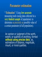
To determine possible accuracy of estimation
with given presice level, we need to know
distribution of the estimation
Normally it is very hard to determine exactly the
real value of concerned parameter. The one must

estimate the value by using some suitable
method

Meet with some error in estimation

Need to evaluate accuracy of estimation: with
a given precise level the estimation result is
acceptable or not?




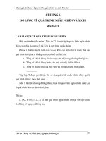
Distribution of variable
Distribution of variable
The set of values of a set of data, possibly grouped into
The set of values of a set of data, possibly grouped into
classes, together with their frequencies or relative
classes, together with their frequencies or relative
frequencies
frequencies
Distribution of variable: the set of possible values with
Distribution of variable: the set of possible values with
their probability
their probability




Example
Example

:
:
-
-
Tossing a coin:
Tossing a coin:
Possibility to get “figure side“
Possibility to get “figure side“
=
=
1/2
1/2




uniform distribution of two values
uniform distribution of two values
“figure side“ and “number side“
“figure side“ and “number side“
-


Tossing a dice:
Tossing a dice:
Probability to get the side with
Probability to get the side with
six points =
six points =
1/6

1/6




uniform distribution of 6
uniform distribution of 6
values * , ** , *** , **** , ***** and ******
values * , ** , *** , **** , ***** and ******
-
Tossing 6 dices:
Tossing 6 dices:
Non-uniform distribution of 36
Non-uniform distribution of 36
values 6* , 7* , 8* , “ , 35* and 36*
values 6* , 7* , 8* , “ , 35* and 36*




Concept of probability distribution
Concept of probability distribution
* Discrete distributions:
* Discrete distributions:
Variable X with
Variable X with


Value:
Value:

X1 X2 X3 . . . Xn
X1 X2 X3 . . . Xn


| | | |
| | | |
Probability:
Probability:
p1 p2 p3 pn
p1 p2 p3 pn


P {X=X1} = p1 >= 0
P {X=X1} = p1 >= 0


P {X=X2} = p2 >= 0
P {X=X2} = p2 >= 0


. . .
. . .


P {X=Xn} = pn >= 0
P {X=Xn} = pn >= 0

p1 + p2 + . . . + pn = 1 (100%)
p1 + p2 + . . . + pn = 1 (100%)




Concept of probability distribution
Concept of probability distribution
* Discrete distributions:
* Discrete distributions:


p6
p6




p3
p3


p2
p2


p1
p1

x1 x2 x3 xn
x1 x2 x3 xn




Concept of probability distribution
Concept of probability distribution
* Continuous distributions:
* Continuous distributions:
Variable X taken value x inside interval (a;b) with density function f(x) >= 0
Variable X taken value x inside interval (a;b) with density function f(x) >= 0
( ) 1 ; - b +
b
a
f x dx a= ∞ ≤ < ≤ ∞
∫
{ ( ; )} ( ) for
d
c
P X c d f x dx a c d b∈ = ≤ < ≤
∫




Concept of probability distribution
Concept of probability distribution
* Continuous distributions:
* Continuous distributions:

Estimation of rate (proportion, probability)
Estimation of rate (proportion, probability)
In study population let“s consider a binary variable
In study population let“s consider a binary variable
X
X


with 2 values
with 2 values
0
0
and
and
1
1
Suppose
Suppose
X
X
takes value
takes value
1
1
with rate
with rate

(proportion,
(proportion,
probability
probability
)
)
p
p
and value
and value
0
0


with rate
with rate
1 “ p
1 “ p
, where
, where
p
p
is
is
unknown (0 <
unknown (0 <
p
p

<1)
<1)
Usually we estimate the rate
Usually we estimate the rate
p
p
by taking a sample of the
by taking a sample of the
variable
variable
X
X
with
with
n
n
observations
observations
x(1), x(2), “ , x(n)
x(1), x(2), “ , x(n)
.
.
Then determine the number
Then determine the number
m(p)
m(p)
of values
of values
1
1

among the
among the
n
n
observations and perform the proportion
observations and perform the proportion


m(p) / n
m(p) / n


as an estimated value of the rate
as an estimated value of the rate
p
p
.
.
That way of estimation is “reasonable “ or not?
That way of estimation is “reasonable “ or not?


The theorem proved mathematically shows the
taking the proportion m(p) / n for estimation of
the rate p is completely “reasonable”: we can
get the “true” rate when the sample size is very
large.
THEOREM (louvlier). The proportion
m(p) / n
m(p) / n

tends to p when n tens to infinity (is very large).

Distribution of
Distribution of
sample
sample
rate (proportion)
rate (proportion)
Let
Let
X
X
be a binary variable taken value
be a binary variable taken value
1
1
with
with
unknown probability
unknown probability
p
p
and taken value
and taken value
0
0
with
with
probability
probability

1 “ p
1 “ p
(Bernoulli“s distribution).
(Bernoulli“s distribution).
Estimating
Estimating
p
p
: perform a sample
: perform a sample
x(1), x(2), “ , x(n)
x(1), x(2), “ , x(n)
of
of
X
X and take


m(p) / n
m(p) / n
as an estimation of
as an estimation of
p
p


(m(p) = number of
(m(p) = number of
1“s
1“s

appeared in the sample).
appeared in the sample).
Quantity
Quantity
m(p) / n
m(p) / n
should take values
should take values


0/n , 1/n , 2/n , “ , (n-1) / n , n/n
0/n , 1/n , 2/n , “ , (n-1) / n , n/n
,
,
each with certain “possibility“ (probability)
each with certain “possibility“ (probability)

Distribution of
Distribution of
sample
sample
rate (proportion)
rate (proportion)
Quantity
Quantity
m(p) / n
m(p) / n
is a random variable with
is a random variable with
binomial distribution

binomial distribution
with parameters
with parameters
p
p
and
and
n
n
.
.




Binomial Distribution
Binomial Distribution


Parameters of binomial distribution are the rate
Parameters of binomial distribution are the rate
p
p
and number
and number
n
n
of experiments
of experiments
0

0
1
1
8
8
9
9
7
7
6
6
5
5
4
4
3
3
2
2
{ } ( )
( ) 1 ; 0,1,2, ,
−
= = − =
n k
k k
n
P m p k C p p k n

Distribution of
Distribution of

sample
sample
rate (proportion)
rate (proportion)

Binomial distribution can be used to evaluate
error in estimating p by m(p) / n



For small
For small
n
n
, calculation with binomial
, calculation with binomial
distribution is practicable
distribution is practicable



For
For
n
n
large the calculation is very cumbersome
large the calculation is very cumbersome


need to have another method for evaluation

need to have another method for evaluation

Distribution of
Distribution of
sample
sample
rate (proportion)
rate (proportion)
moivre-laplace theorem. Let


X
X
be a
be a
binary variable taken value
binary variable taken value
1
1
with probability
with probability
p
p


and value
and value
0
0
with probability

with probability
1 “ p
1 “ p
. For the
. For the
sample
sample
x(1), x(2), “ , x(n)
x(1), x(2), “ , x(n)
of
of
X
X
with
with
n
n


observation let
observation let
m(p) / n
m(p) / n
be the proportion 1“s
be the proportion 1“s
number per sample size. Then the proportion is a
number per sample size. Then the proportion is a
quantity with distribution approximate to
quantity with distribution approximate to
Normal

Normal
distribution
distribution
with mean value (expectation)
with mean value (expectation)
p
p
and
and
variance
variance
p . (1-p) / n
p . (1-p) / n
when the sample size
when the sample size
n
n
is
is
large.
large.




Normal distribution (Gauss distribution)
Normal distribution (Gauss distribution)
Normal distribution defined by its “expectation” vµ “variance”
Normal distribution defined by its “expectation” vµ “variance”
( )

2
2
1
( )
2
x
f x exp
µ
πσ
σ
 
−
 ÷
= −
 ÷
 

Distribution of
Distribution of
sample
sample
rate (proportion)
rate (proportion)

Moivre-Laplace Theorem can be used to evaluate errors in estimation
of proportion:
allows to determine Confidence Interval of the estimation

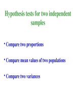
Confidence interval of estimation
Confidence interval of estimation

(interval estimation)
(interval estimation)

For a variable with normal distribution with
expectation p and variance p . (1-p) / n
95% Confidence Interval of estimation of p is the
interval

Confidence Interval
Confidence Interval
of estimation is an interval
of estimation is an interval
containing the estimated value of parameter,
containing the estimated value of parameter,
informing the
informing the
true value
true value
of parameter can be some
of parameter can be some
point inside the interval with given probability
point inside the interval with given probability
a
a
.
.
( 1.96* .(1 ) / ; 1.96* .(1 ) / )p p p n p p p n− − + −

Confidence interval of proportion
Confidence interval of proportion

Because estimation of proportion (by Moivre “
Laplace Theorem) is a quantity with distribution
approximate to Normal Distribution, 95%
Confidence Interval of proportion estimation is
where
ˆ ˆ ˆ ˆ ˆ ˆ
1.96* .(1 ) / 1.96* .(1 ) /;p p p n p p p n
 
− − + −
 
ˆ
( ) /p m p n=

Application
Application
Problem: How to estimate the amount of fishes
in a lake?
Step 1.
Step 1.
The amount of fishes in a lake is
The amount of fishes in a lake is
N
N
=?
=?
•
Nesting 1st time to capture certain amount
Nesting 1st time to capture certain amount
m1
m1

of fishes
of fishes
•
Mark each fish of that amount. Then release
Mark each fish of that amount. Then release
those fishes back into the lake. Hence the true
those fishes back into the lake. Hence the true
proportion of marked fishes in the lake equals
proportion of marked fishes in the lake equals
p = m1 / N
p = m1 / N

Step 2.
Step 2.
Nesting 2nd time to capture another
Nesting 2nd time to capture another
amount
amount
n
n
of fishes
of fishes
•
Count the amount
Count the amount
m2
m2
of marked fishes

of marked fishes
among
among
n
n
fishes captured in the 2nd time
fishes captured in the 2nd time
•
Estimate the proportion
Estimate the proportion
p
p
of marked fishes
of marked fishes
by
by
p“ = m2 / n
p“ = m2 / n
with 95% confidence interval
with 95% confidence interval
' 1.96* '.(1 ') / ' 1.96* '.(1; ') /p p p n p p p n
 
− − + −
 

Step 3.
Step 3.
We are sure (with 95% possibility) that the true
We are sure (with 95% possibility) that the true
proportion

proportion
p
p
of marked fishes in the lake should be a
of marked fishes in the lake should be a
certain number inside the confidence interval, that means
certain number inside the confidence interval, that means


We can be sure (with 95% certainty) that the amount of
We can be sure (with 95% certainty) that the amount of
fishes in the lake should be a number between
fishes in the lake should be a number between
1/ ' 1.96* '.(1 ') / ;
1/ ' 1.96* '.(1 ') /
p m N p p p n
p m N p p p n
= ≥ − −
= ≤ + −
1/( ' 1.96* '.(1 ') / )
1/( ' 1.96* '.(1 ') / )
m p p p n N
N m p p p n
+ − ≤
≤ − −

For estimation of expectation of a quantitative
For estimation of expectation of a quantitative
variable
variable

X
X
, a sample
, a sample
x(1), x(2), “ , x(n)
x(1), x(2), “ , x(n)
can be
can be
chosen and
chosen and
sample mean value
sample mean value
(sample average)
(sample average)
Can be taken as an estimated value of
Can be taken as an estimated value of
expectation
expectation
parameter E(X)
parameter E(X)
of
of
X
X





That manner (of estimation) is correct or not?
That manner (of estimation) is correct or not?
1
( (1) (2) ( ))X x x x n
n
= + + +
Estimation of Expectation
Estimation of Expectation
Expectation of variable
Expectation of variable


=
=


Mean value of variable in whole population
Mean value of variable in whole population