Tài liệu Slide bài giảng môn Lý thuyết xác suất thống kê bằng Tiếng Anh StatisticsLecture4A_HypothesisTest

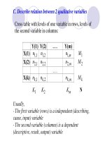
Hypothesis Test
“ Hypothesis Test”: A procedure for
deciding between two hypotheses (null
hypothesis – alternative hypothesis) on the
basis of observations in a random sample

One sample Hypothesis test–
•
Compare proportion to a given value of rate
•
Compare mean value to a given value of
expectation



Test 1. Compare proportion to a given rate
- a sample of n independent observations
collected from a binary variable X taking value 1 with
(unknown) probability p (0 < p < 1) and value 0 with
probability 1 p–  Given a number q , how to have a
conclusion comparing p with q based on information
of the sample?
(Null) Hypothesis
H: p = q
Alternative Hypothesis
K: p differs from q
(Two tails Hypothesis Test)
1 2
( , , , )
n

X X X

Solution
By Moivre-Laplace Theorem, for large sample
size, sample proportion m(p)/n of appearance
of number 1 has distribution approximate to
normal distribution with expectation p and
variance p . (1-p) / n . Then a testing
procedure can be as follows:
Step 1. Estimate a sample proportion by
p = m(p) / n’

Step 2.
Version A (by computer): Calculate the
probability (using normal distribution with
expectation




p’
p’
and variance
and variance
p . (1-p ) / n’ ’
p . (1-p ) / n’ ’ )
such that a estimate point should appear at a
location with distance to the p’ longer than
| q p– ’ |
= Probability b (called p-value) of wrong decision

of excluding estimation value q (saying that q
differs from true value of p) when this value should
be a “good” value of estimation


Step 3. Compare b with a given confidence
level alpha (5%, 1%, 0.5% or 0.1%)
•
If b < alpha  reject the hypothesis H,
conclude that q differs from p , because
possibility of getting mistake in decision is “very
small”
* If b > alpha  accept the hypothesis H,
confirm q = p , because possibility of having
mistake by rejecting the hypothesis is too large


Version B. (Calculate by hand, using critical value)
Using Table of Normal Distribution to have a
critical value Z(alpha/2) with given confidence
level alpha (5%, 1% or 0.5%, for alpha = 5% we
have Z(alpha/2) = 1.96) and calculate the value
Decide
Reject the Hypothesis H if U > Z(alpha/2)
Accept the Hypothesis H if U =< Z(alpha/2)
| ' | / '.(1 ') /U p q p p n
 
= − −
 

Version C. Using confidence intervals
With confidence level of 5%, we can use
confidence intervals for hypothesis testing:
Decide
•
Reject the Hypothesis H if the confidence
interval does not contain the point q
•
Accept the Hypothesis H if the confidence
interval contains the point q
' 1.96* '.(1 ') / ; ' 1.96* .(1 ) /p p p n p p p n
 
− − + −
 

Test 1A. Compare proportion to a given value -
One-tail test
Null Hypothesis
H: q = p
Alternative Hypothesis
K: q > p
With a sample of n independent observations
collected from a binary variable X taking value 1
with (unknown) probability p (0 < p < 1) and
value 0 with probability 1 p–  Given a
number q , can we conclude that p < q?

Steps of testing
Step 1. Estimate sample proportion by
p = m(p) / n’

Step 2. Using normal distribution (with
expectation
p’
p’

and variance
p . (1-p ) / n’ ’
p . (1-p ) / n’ ’ )
calculate the probability
of estimation value
of estimation value
being greater than
being greater than q .
= probability b of those estimated values which
should be rejected by chance

Step 3 Compare b to a given confidence level
alpha (5%, 1%, 0.5% or 0.1%)
•
If b < alpha  reject the hypothesis H and
confirming q > p (because probability to get
wrong conclusion is small enough)
* If b > alpha  accept the hypothesis H,
confirming q = p , (because possibility to meet
mistake accepting q > p should be too large)



Note 1
For Hypothesis

H: q = p
with Alternative Hypothesis
K: q < p
the testing procedure is exactly the same

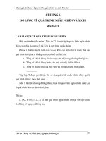
Test 2. Compare mean value to a given value of
expectation
Problem: Taking a sample from a variable X
with normal distribution (or sample size be
large), we need to compare the sample mean
Mean(X) to a given value a. Then there are 3
types of test
A. Two-tail Test: Hypothesis
H: Mean(X) = a
Alternative Hypothesis
K: Mean(X) differs from a

B. “Right hand side” One-tail Test:
Hypothesis
H: Mean(X) = a
Alternative Hypothesis
K: Mean(X) > a
C. “Left hand side” One-tail Test: Hypothesis
H: Mean(X) = a
Alternative Hypothesis
K: Mean(X) < a

For testing the above hypothesis, the distribution of
sample mean value must be known. Meantime the
variance of the variable X is unknown and must be

estimated. Then the following theorem can be applied:
1
.( )
n
t X
S
µ
−
= −
1 2
( , , , )
n
X X X
Theorem. Let be a sample of n
independent observations taken from a normal distributed
variable X with expectation , is sample mean value
and is sample variance. Then the (new) variable
has T-Student distribution with (n-1) degrees of freedom.
X
µ
2
S

Remark. By Central Limit Theorem, when sample
size is large, distribution of sample mean value is
approximate to normal distribution. Then the
above theorem can be applied also for testing
hypothesis comparing mean value of variable with
non-normal distribution

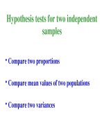
Student (T) distribution
Parameter of Student Distribution: “Degree of Fredom”
ν

Steps of Testing
Step 1. Estimate sample Mean Value Mean(X)
Standard Deviation SD(X)
Step 2. Calculate the statistic
where n is sample size and a is the given value to
which the mean value has be compared
1.( ( ) )
( )
( )
n Mean X a
t a
SD X
− −
=

Step 3 (Version A – by computer). Taking a Student
distribution variable T(n-1) with (n-1) degree of freedom
and calculate the probability
b = P{ | T(n-1) | >= | t(a) | }
for two-tails test,
b = P { T(n-1) >= t(a) }
for right side one-tail test, and
b = P { T(n-1) =< t(a) }
for left side one-tail test (then t(a) < 0 )

Step 4. Compare the probability b with a given ahead level

of significance alpha (= 5%, 1%, 0.5%, 0.1%, etc.):
If b >= alpha  accept the hypothesis H , conclude
Mean(X) = a
If b < alpha  reject the hypothesis H :
-
Declare Mean(X) differs from a (for the two+tails
test)
-
Declare Mean(X) > a (for right side one-tail test)
-
Declare Mean(X) < a (for left side one-tail test)