Output Tracking with Discrete-Time Integral Sliding Mode Control

Output Tracking with Discrete-Time Integral
Sliding Mode Control
Xu Jian-Xin and Khalid Abidi
Department of Electrical and Computer Engineering, National University of
Singapore, 4 Engineering Drive 3, Singapore 117576
{elexujx,kabidi}@nus.edu.sg
1 Introduction
Sliding mode control is a very popular robust control method owing to its ease
of design and robustness to “matched” disturbances. However, full state infor-
mation is required in the controller design which is a drawback since in most
practical applications only the output measurement is available. To solve this
problem, focus was placed on output feedback based sliding mode control [1]-
[6]. Two approaches arose: a design based on observers to construct the missing
states, [3],[4], the other design focused on using only the output measurement,
[1],[2]. Both approaches present certain strengths and limitations.
Computer implementation of control algorithms presents a great convenience
and has, hence, caused the research in the area of discrete-time control to in-
tensify. This also necessitated a rework in the sliding mode control strategy for
sampled-data systems. Most of the discrete-time sliding mode approaches are
based on the availability of full state information, [7]-[9]. A few approaches did
focus on the output measurement, [5],[6]. In [5],[6], the control design was based
on the assumption that the state matrix of a discrete-time system is invert-
ible. This is true for sampled-data systems. In this chapter we will focus on
state based approaches as well as expand upon the work of [5],[6] by focusing
on arbitrary reference tracking of a linear time invariant system with matched
disturbance.
A delay in the state or disturbance estimation in sampled-data systems is an
inevitable phenomenon and must be studied carefully. In [9] it was shown that
in the case of delayed disturbance estimation a worst case accuracy of O(T )
can be guaranteed for deadbeat sliding mode control design and a worsted case
accuracy of O(T

2
) for integral sliding mode control. While deadbeat control
is a desired phenomenon, it is undesirable in practical implementation due to
the over large control action required. In [9] the integral sliding mode design
avoided the deadbeat response by eliminating the poles at zero. A similar effect
is possible in an integral sliding mode design for output tracking.
This chapter considers the output tracking of a minimum-phase linear sys-
tem subject to matched time varying disturbance. To accomplish the task of
G. Bartolini et al. (Eds.): Modern Sliding Mode Control Theory, LNCIS 375, pp. 247–268, 2008.
springerlink.com
c
 Springer-Verlag Berlin Heidelberg 2008
248 X. Jian-Xin and K. Abidi
arbitrary reference tracking three approaches will be considered: 1) State Feed-
back, 2) Output Feedback, and 3) Output Feedback with a State Observer.
In each approach the objective is to drive the output tracking error to a cer-
tain neighborhood of the origin. For this purpose a discrete-time integral sliding
surface (ISM) is proposed. The proposed scheme allows full control of the closed-
loop error dynamics and the elimination of the reaching phase. The elimination
of deadbeat response helps in avoiding the generation of over large control in-
puts. It is also worth to highlight that the discrete-time integral sliding mode
control (ISMC) can achieve the O(T
2
) boundary for output tracking error even
in the presence of O(T ) accuracy in the state estimation.
2 Problem Formulation
Consider the following minimum-phase continuous-time system with a nominal
linear time invariant model and matched disturbance
˙
x(t)=Ax(t)+B(u(t)+f(t))

y(t)=Cx(t)
(1)
where the state x ∈
n
, the output y ∈
m
,thecontrolu ∈
m
,andthedis-
turbance f ∈
m
is assumed smooth and bounded. The discretized counterpart
of (1) can be given by
x
k+1
= Φx
k
+ Γ u
k
+ d
k
y
k
= Cx
k
, y
0
= y(0)
(2)
where

Φ = e
AT
,Γ=

T
0
e
Aτ
dτB
d
k
=

T
0
e
Aτ
Bf((k +1)T − τ )dτ ,
and T is the sampling period. (Φ, Γ, C) are controllable and observable. Here the
disturbance d
k
represents the influence accumulated from kT to (k +1)T ,inthe
sequel it shall directly link to x
k+1
= x((k +1)T). From the definition of Γ it
can be shown that
Γ = BT +
1
2!
ABT

2
+···= BT +MT
2
+O(T
3
) ⇒ BT = Γ −MT
2
+O(T
3
)(3)
where M is a constant matrix because T is fixed. From (3), it can be concluded
that the magnitude of Γ is O(T ).
The control objective is to design a discrete-time integral sliding manifold
and a discrete-time SMC law that will stabilize the sampled-data system (2)
and achieve as precisely as possible output tracking. Meanwhile the closed-loop
Output Tracking with Discrete-Time Integral Sliding Mode Control 249
dynamics of the sampled-data system has m closed-loop poles assigned to desired
locations.
In [9] it was shown that as a consequence of sampling, the disturbance orig-
inally matched in continuous-time will contain mismatched components in the
sampled-data system. This is summarized in the following relation, [9],
d
k
=

T
0
e
Aτ
Bf((k +1)T − τ )dτ = Γ f

k
+
1
2
Γ v
k
T + O(T
3
)(4)
where v
k
= v(kT ), v(t)=
d
dt
f(t), d
k
= O(T ), d
k
− d
k−1
= O(T
2
), and d
k
−
2d
k−1
+ d
k−2
= O(T

3
). Note that the magnitude of the mismatched part in the
disturbance d
k
is of the order O(T
3
).
3 Output Tracking ISM: State Feedback Approach
3.1 Controller Design
Consider the discrete-time integral sliding-surface defined below,
σ
k
= e
k
− e
0
+ ε
k
ε
k
= ε
k−1
+ Ee
k−1
(5)
where e
k
= r
k
−y

k
is the tracking error, r
k
is the reference trajectory, y
k
is the
output, σ
k
, 
k
∈
m
are the sliding function and integral vectors, e
0
is the intial
error, and E ∈
m×m
is the design matrix. The output tracking problem is to
force y
k
→ r
k
.
To proceed with the controller design, consider a forward expression of (5)
σ
k+1
= e
k+1
− e
0

+ ε
k+1
ε
k+1
= ε
k
+ Ee
k
.
(6)
Substituting ε
k+1
and (2) into the expression of the sliding surface in (6) and
equating σ
k+1
to zero leads to
σ
k+1
= e
k+1
+ Ee
k
− e
0
+ ε
k
= e
k+1
− (I
m

− E)e
k
+ σ
k
=0 (7)
where I
m
is a unity matrix of dimension m. If we substitute y
k+1
= CΦx
k
+
CΓu
k
+ Cd
k
into (7) and solve for the equivalent control u
eq
k
we have
u
eq
k
=(CΓ)
−1
[r
k+1
− Λe
k
− CΦx

k
− Cd
k
+ σ
k
](8)
where Λ = I
m
− E. Under the assumptions made, the control cannot be im-
plemented in the same form as in (8) because of the lack of knowledge of the
disturbance d
k
. To overcome this, the disturbance estimate will be used. There-
fore, the final controller structure is given by
u
k
=(CΓ)
−1

r
k+1
− Λe
k
− CΦx
k
− C
ˆ
d
k−1
+ σ

k

(9)
where
ˆ
d is the disturbance estimate and in the case of full state availability the
following delay based estimation can be used, [7],
250 X. Jian-Xin and K. Abidi
ˆ
d
k−1
= d
k−1
= x
k
− Φx
k−1
− Γ u
k−1
. (10)
Once the controller is designed, we need to examine the closed-loop state and
output stability.
3.2 Stability Analysis
In order to derive the closed-loop state dynamics we substitute u
k
defined by
(9) into (2) and obtain the following
x
k+1
=


Φ − Γ (CΓ)
−1
(CΦ −ΛC)

x
k
+ d
k
− Γ (CΓ)
−1
C
ˆ
d
k−1
+Γ (CΓ)
−1
(r
k+1
− Λr
k
)+Γ (CΓ)
−1
σ
k
.
(11)
Since, the difference between u
eq
k

and u
k
is the substitution of d
k
with
ˆ
d
k−1
the
sliding surface σ
k+1
will no longer be zero but rather a function of the difference
d
k
−
ˆ
d
k−1
as follows
σ
k+1
= C(
ˆ
d
k−1
− d
k
) (12)
Thus, we obtain the closed-loop state dynamics during sliding mode. In order to
conclude on the stability of (11) we propose the following Lemma.

Lemma 1. The eigenvalues of

Φ −Γ(CΓ)
−1
(CΦ −ΛC)

are the eigenvalues
of Λ and the non-zero eigenvalues of [Φ − Γ (CΓ)
−1
CΦ].
Proof: See Appendix.
According to Lemma 1 the matrix

Φ − Γ (CΓ)
−1
(CΦ −ΛC)

has m poles to
be placed at desired locations while the remaining n −m poles are the open-loop
zeros of the system. Since, the system (2) is assumed to be minimum phase,
the fixed n − m poles are stable. Therefore, stability of the closed-loop state
dynamics is guaranteed.
Substitution of (11) into y
k+1
yields the dynamics
y
k+1
= −Λe
k
+ r

k+1
+ Cd
k
− C
ˆ
d
k−1
+ σ
k
. (13)
Substituting the result σ
k
= C(
ˆ
d
k−2
− d
k−1
) obtained from (12) into (13)
y
k+1
= −Λe
k
+ r
k+1
+ C(d
k
−
ˆ
d

k−1
− d
k−1
+
ˆ
d
k−2
). (14)
This yields the tracking error dynamics,
e
k+1
= Λe
k
+ δ
k
(15)
where δ
k
is given by
δ
k
= −C(d
k
−
ˆ
d
k−1
− d
k−1
+

ˆ
d
k−2
). (16)
Remark 1. From (15) we see that the reference tracking dynamics depends on
thechoiceofΛ which is a design matrix. However, internal stability require that
Output Tracking with Discrete-Time Integral Sliding Mode Control 251
the open-loop zeros of the system are stable and, thus, it should be minimum
phase.
3.3 Tracking Error Bound
In order to calculate the tracking error bound we must find the bound of δ
k
.
Looking back at (16), δ
k
was given by
δ
k
= −C(d
k
−
ˆ
d
k−1
− d
k−1
+
ˆ
d
k−2

). (17)
From (10)
ˆ
d
k−1
= d
k−1
, therefore, (17) becomes
δ
k
= −C(d
k
− d
k−1
− d
k−1
+ d
k−2
). (18)
which simplifies to
δ
k
= −C(d
k
− 2d
k−1
+ d
k−2
). (19)
In [9] it is shown that d

k
− 2d
k−1
+ d
k−2
= O(T
3
) if the smoothness and
boundedness conditions on f(t) hold. Therefore,
δ
k
= −C(d
k
− 2d
k−1
+ d
k−2
)=O(T
3
). (20)
According to [9] the ultimate error bound on e
k
 will be one order higher than
the bound on δ
k
due to convolution and since the bound on δ
k
is O(T
3
)the

ultimate bound on e
k
 is O(T
2
). Thus, the ultimate bound on the tracking
error is
e
k
 = O(T
2
). (21)
4 Output Tracking ISM: Output Feedback Approach
4.1 Controller Design
In most practical situations, full state measurement is not possible and only the
output is measured. Thus, it makes more sense to try to derive a controller that
is a function of the output tracking error.
In order to proceed we will first define the reference model
x
r,k+1
=

Φ − Γ (CΓ)
−1
CΦ

x
r,k
+ Γ (CΓ)
−1
r

k+1
y
r,k
= Cx
r,k
= r
k
(22)
where x
r,k
∈
n
is the reference model state vector, y
r,k
∈
m
is the reference
model output vector, and r
k
∈
m
is the reference trajectory. Due to the dead-
beat nature of the reference model its output is the desired reference trajectory
r
k
and, therefore, tracking this reference model would lead to the desired re-
sponse. The only drawback is that the stability of the reference model requires
that the system (2) satisfy the minimum phase condition. Now define D = CΦ
−1
,

consider the sliding surface
252 X. Jian-Xin and K. Abidi
σ
k
= D [x
r,k
− x
k
]+ε
k
ε
k
= ε
k−1
+ ED [x
r,k−1
− x
k−1
]
(23)
where D eliminates the state dependency, σ
k
, ε
k
∈
m
are the sliding function
and integral vectors, and E ∈
m×m
is a design matrix of rank m. The design

associated with D is adopted in [5],[6]. Note that unlike the sliding surface (5)
which is based on the output y
k
, sliding surface (23) is based on the states
x
k
. To proceed with the design consider a forward expression of the sliding
surface (23)
σ
k+1
= D [x
r,k+1
− x
k+1
]+ε
k+1
ε
k+1
= ε
k
+ ED [x
r,k
− x
k
]
(24)
Substituting the sampled-data system (2) into (24)
σ
k+1
= D [x

r,k+1
− Φx
k
− Γ u
k
− d
k
]+ε
k+1
ε
k+1
= ε
k
+ ED [x
r,k
− Φx
k−1
− Γ u
k−1
− d
k−1
]
(25)
From the definition of D we have DΦx = y, therefore, we can eliminate x from
(25) resulting in the expression for the sliding surface
σ
k+1
= Dx
r,k+1
− y

k
− DΓu
k
− Dd
k
+ ε
k+1
(26)
and the expression for the integral variable ε
k+1
ε
k+1
= ε
k
+ E [Dx
r,k
− y
k−1
− DΓu
k−1
− Dd
k−1
] . (27)
Sliding mode condition occurs when σ
k+1
= 0, therefore, setting the right-hand
side of (26) to zero and solving for the equivalent control u
eq
k
,weget

u
eq
k
=(DΓ )
−1
[Dx
r,k+1
− y
k
− Dd
k
+ ε
k+1
] (28)
and ε
k+1
is found from (27). Controller (28) is not practical as it requires apriori
knowledge of the disturbance. Thus, the estimate of the disturbance will be used.
However, note that the disturbance estimate used in the state feedback controller
designed in Section 3 requires full state information which is not available in this
case. Therefore, an observer that is based on output feedback will have to be
used. If we substitute the delayed disturbance estimate,
ˆ
d
k−1
, instead of d
k
the
final controller becomes
u

k
=(DΓ )
−1

Dx
r,k+1
− y
k
− D
ˆ
d
k−1
+ ε
k+1

(29)
and the expression for the integral variable (27) becomes
ε
k+1
= ε
k
+ E

Dx
r,k
− y
k−1
− DΓu
k−1
− D

ˆ
d
k−1

(30)
where the disturbance estimate
ˆ
d
k
based on output information will be given in
subsection 4.3.
Output Tracking with Discrete-Time Integral Sliding Mode Control 253
4.2 Stability Analysis
With the controller design, the stability of the closed-loop system must be an-
alyzed. For this we will substitute (30) in (29) and substitute the resulting ex-
pression for u
k
into (2) leading to the closed-loop equation during sliding mode,
x
k+1
= Φx
k
− Γ (DΓ )
−1
[y
k
+ E (y
k−1
+ DΓu
k−1

)] + d
k
−Γ (DΓ )
−1
[D + ED]
ˆ
d
k−1
+ Γ (DΓ )
−1
[Dx
r,k+1
+ EDx
r,k
+ ε
k
]
(31)
To get the state dynamics, y
k
will be replaced by DΦx
k
and [y
k−1
+ DΓu
k−1
]
will be replaced by [Dx
k
− Dd

k−1
] and the result is simplified
x
k+1
=

Φ −Γ(DΓ)
−1
(DΦ + ED)

x
k
+ d
k
− Γ (DΓ )
−1
D
ˆ
d
k−1
+Γ (DΓ )
−1
[Dx
r,k+1
+ EDx
r,k
+ ε
k
+ ED(d
k−1

−
ˆ
d
k−1
)] (32)
Solving ε
k
in (23) in terms of x
r,k
, x
k
and σ
k
ε
k
= σ
k
− D(x
r,k
− x
k
) (33)
and substituting into (32) the following closed-loop dynamics is obtained
x
k+1
=

Φ − Γ (DΓ )
−1
(DΦ − ΛD)


x
k
+ d
k
− Γ (DΓ )
−1
D
ˆ
d
k
+Γ (DΓ )
−1
[Dx
r,k+1
− ΛDx
r,k
+ ED(d
k−1
−
ˆ
d
k−1
)+σ
k
]. (34)
where Λ = I
m
−E. Further, it can be shown that the expression of σ
k+1

in (24)
is of the form
σ
k+1
= D(d
k
−
ˆ
d
k−1
)+ED(d
k−1
−
ˆ
d
k−1
) (35)
We see from (35) that σ
k+1
is a function of d and
ˆ
d. It will be shown later
that the disturbance observer is not dependent on the state dynamics and, thus,
σ
k+1
is not coupled to x
k+1
. Using a delayed form of (35), σ
k
= D(d

k−1
−
ˆ
d
k−2
)+ED(d
k−2
−
ˆ
d
k−2
)in(34)weobtain
x
k+1
=

Φ − Γ (DΓ )
−1
(DΦ − ΛD)

x
k
+Γ (DΓ )
−1
[Dx
r,k+1
−ΛDx
r,k
]+ζ
k

(36)
where
ζ
k
= d
k
− Γ (DΓ )
−1
D(
ˆ
d
k−1
+ d
k−1
−
ˆ
d
k−2
)
+Γ (DΓ )
−1
ED(d
k−1
−
ˆ
d
k−1
+ d
k−2
−

ˆ
d
k−2
).
Subtracting both sides of (36) from x
r,k+1
yields
x
r,k+1
− x
k+1
= −

Φ − Γ (DΓ )
−1
(DΦ − ΛD)

x
k
+[I −Γ (DΓ)
−1
D]x
r,k+1
+ Γ (DΓ )
−1
ΛDx
r,k
− ζ
k
(37)

254 X. Jian-Xin and K. Abidi
finally substituting (22) into the r.h.s of (37) and using the fact that [I −
Γ (DΓ )
−1
D]Γ =0weobtain
Δx
k+1
=

Φ − Γ (DΓ )
−1
(DΦ − ΛD)

Δx
k
− ζ
k
. (38)
where Δx = x
r
− x.FromLemma 1 the closed-loop poles of (38) are the
eigenvalues of Λ and the open-loop zeros of the system (Φ, Γ, D). Thus, m poles
of the closed-loop system can be selected by the proper choice of the matrix Λ
while the remaining poles are stable only if the system (Φ, Γ, D) is minimum
phase.
We have established the stability condition for the closed-loop system, but,
have not yet established the tracking error bound. For this we need to first discuss
the disturbance estimate
ˆ
d

k
upon which the tracking error bound depends. The
next section will address this.
4.3 Disturbance Observer Design
In order to design the observer we first need to note that according to (4) the
disturbance can be written as
d
k
= Γf
k
+
1
2
Γ v
k
T + O(T
3
)=Γ η
k
+ O(T
3
) (39)
where η
k
= f
k
+
1
2
v

k
T .Ifη
k
can be estimated then the estimation error of d
k
would be O(T
3
) which is acceptable in practical applications. Define the observer
x
d,k+1
= Φx
d,k
+ Γ u
k
+ Γ
ˆ
η
k
y
d,k
= Cx
d,k
(40)
where x
d
∈
n
is the observer state vector, y
d
∈

m
is the observer output
vector,
ˆ
η ∈
m
is the disturbance estimate and will act as the “control input”
to the observer, therefore the estimate
ˆ
d
k
= Γ
ˆ
η
k
. Since the disturbance estimate
will be used in the final control signal it must not be overly large, therefore, it is
wise to avoid a deadbeat design. For this reason we will use an observer based
on an integral sliding surface
σ
d,k
= e
d,k
− e
d,0
+ ε
d,k
ε
d,k
= ε

d,k−1
+ E
d
e
d,k−1
(41)
where e
d,k
= y
k
− y
d,k
, is the output estimation error, σ
d
, ε
d
∈
m
are the
sliding function and integral vectors, and E
d
is a design matrix.
Since the sliding surface (41) is the same as (5), by following the derivation
procedure shown in Subsection 3.1, that is, letting σ
d,k+1
=0,weobtain
ˆ
η
k
=(CΓ)

−1
[y
k+1
− Λ
d
e
d,k
− CΦx
d,k
+ σ
d,k
] − u
k
(42)
where Λ
d
= I
m
− E
d
. Expression (42) is the required disturbance estimate and
is similar in form to (8). Note, however, that (42) requires the future value of
the output y
k+1
which is not possible therefore the delayed (42) is used
Output Tracking with Discrete-Time Integral Sliding Mode Control 255
ˆ
η
k−1
=(CΓ)

−1
[y
k
− Λ
d
e
d,k−1
− CΦx
d,k−1
+ σ
d,k−1
] − u
k−1
. (43)
Since, only
ˆ
η
k−1
is available the observer model (40) will be delayed as well.
Substitution of (43) into the delayed form of (40) and following the same steps
of the derivation of (11) we obtain
x
d,k
=

Φ − Γ (CΓ)
−1
(CΦ −Λ
d
C)


x
d,k−1
+ Γ (CΓ)
−1
[y
k
− Λ
d
y
k−1
]. (44)
Subtracting (44) from a delayed form of the system (2) and substituting d
k−1
=
Γ η
k−1
we obtain
Δx
d,k
=

Φ − Γ (CΓ)
−1
(CΦ −ΛC)

Δx
d,k−1
(45)
where Δx

d,k
= x
k
− x
d,k
. The solution of (45) is given by
Δx
d,k−1
=

Φ −Γ(CΓ)
−1
(CΦ −Λ
d
C)

k−1
Δx
d,0
(46)
If we set E
d
= I
m
−Λ
d
where Λ
d
is a diagonal matrix it is shown in Lemma 1
that the poles of the closed-loop system (45) are the eigenvalues of Λ

d
and the
non-zero eigenvalues of [Φ − Γ (CΓ)CΦ]. In control applications, we can choose
eigenvalues Λ
d
closer to origin comparing with the controller eigenvalues Λ.
Premultliplication of (45) with C yields
e
d,k
= Λ
d
e
d,k−1
(47)
Thus, the performance of the observer tracking depends on the choice of Λ
d
.
Finally, we need to look at the disturbance estimation by the observer. For this
we subtract a delayed (40) from a delayed (2) to obtain
Δx
d,k
= ΦΔx
d,k−1
+ Γ (η
k−1
−
ˆ
η
k−1
) (48)

To obtain the η −
ˆ
η relationship, premultiplying both sides of (48) with C and
substituting (47) yield
ˆ
η
k−1
=(CΓ)
−1
(CΦ −Λ
d
C)Δx
d,k−1
+ η
k−1
(49)
or
ˆ
η
k−1
=(CΓ)
−1
(CΦ −Λ
d
C)

Φ − Γ (CΓ)
−1
(CΦ −Λ
d

C)

k−1
Δx
d,0
+ η
k−1
.
(50)
Since

Φ − Γ (CΓ)
−1
(CΦ −Λ
d
C)

is stable, for k large enough

Φ − Γ (CΓ)
−1
(CΦ −Λ
d
C)

k−1
→ 0
and the disturbance estimate will converge to the actual disturbance. As a result,
when k is large enough
d

k
−
ˆ
d
k−1
= Γ(η
k
−
ˆ
η
k−1
)=Γ (η
k
− η
k−1
)=O(T
2
). (51)
256 X. Jian-Xin and K. Abidi
4.4 Tracking Error Bound
Recall that the closed-loop system was in the form
Δx
k+1
=

Φ − Γ (DΓ )
−1
(DΦ − Λ
d
D)


Δx
k
− ζ
k
(52)
and the term ζ
k
was given by
ζ
k
= d
k
− Γ (DΓ )
−1
D(
ˆ
d
k−1
+ d
k−1
−
ˆ
d
k−2
)
+ Γ(DΓ)
−1
ED(d
k−1

−
ˆ
d
k−1
+ d
k−2
−
ˆ
d
k−2
). (53)
Substituting d
k
= Γ η
k
+ O(T
3
)and
ˆ
d
k−1
= Γ
ˆ
η
k−1
we have
ζ
k
= Γ (η
k

−
ˆ
η
k−1
− η
k−1
+
ˆ
η
k−2
)
+ Γ(DΓ)
−1
EDΓ(η
k−1
−
ˆ
η
k−1
+ η
k−2
−
ˆ
η
k−2
)+O(T
3
) (54)
From (50)
ˆ

η
k−1
→ η
k−1
when k is sufficiently large, therefore η
k−1
−
ˆ
η
k−1
+
η
k−2
−
ˆ
η
k−2
→ 0 and (53) renders
ζ
k
= Γ (η
k
− 2η
k−1
+ η
k−2
)+O(T
3
). (55)
Since the disturbance f(t) is assumed smooth and bounded it can be shown that

the magnitude of η
k
− 2η
k−1
+ η
k−2
is O(T
3
). Also since Γ = O(T )
ζ
k
= O(T ) ·O(T
3
)+O(T
3
)=O(T
3
). (56)
According to [9] the ultimate error bound on Δx
k
 will be one order higher
than the bound on ζ due to convolution and since the bound on ζ
k
is O(T
3
)the
ultimate bound on Δx
k
 is O(T
2

). Thus, the ultimate bound on the tracking
error is
e
k
≤CΔx
k
 = O(T
2
). (57)
5 Output Tracking ISM: State Observer Approach
5.1 Controller Structure and Closed-Loop System
In this section we discuss the observer based approach for the unknown states.
Recall that the state based ISM control was given by (8)
u
eq
k
=(CΓ)
−1
[r
k+1
− Λe
k
− CΦx
k
− Cd
k
+ σ
k
] . (58)
Under the assumptions made, the control cannot be implemented in the same

form as in (58) because of the lack of knowledge of the states x
k
as well as
the disturbance d
k
. To overcome this, the state and disturbance estimates ob-
tained from the observers will be used. Therefore, the final controller structure is
given by
Output Tracking with Discrete-Time Integral Sliding Mode Control 257
u
k
=(CΓ)
−1

r
k+1
− Λe
k
− CΦ
ˆ
x
k
− C
ˆ
d
k−1
+ σ
k

. (59)

In order to derive the closed-loop state dynamics we substitute u
k
defined by
(59) into (2),
x
k+1
=

Φ + Γ(CΓ)
−1
ΛC

x
k
− Γ (CΓ)
−1
CΦ
ˆ
x
k
+ Γ (CΓ)
−1
(r
k+1
− Λr
k
)
+Γ (CΓ)
−1
σ

k
+ d
k
− Γ (CΓ)
−1
C
ˆ
d
k−1
.
(60)
To proceed further we assume that the state estimate is related to the actual
state as follows
ˆ
x
k
= x
k
+ κ
k
(61)
where κ
k
is the estimation error. If we substitute (61) in (60) we obtain
x
k+1
=

Φ − Γ (CΓ)
−1

(CΦ −ΛC)

x
k
+ Γ (CΓ)
−1
(r
k+1
− Λr
k
)
+Γ (CΓ)
−1
σ
k
+ d
k
− Γ (CΓ)
−1
C
ˆ
d
k−1
− Γ (CΓ)
−1
CΦκ
k
.
(62)
The sliding surface can similarly be derived as

σ
k+1
= C(
ˆ
d
k−1
− d
k
)+CΦκ
k
. (63)
It will be shown later that the state estimation error κ
k
is not dependent
on the state dynamics x
k
and, thus, the dynamics of the sliding function is
not coupled to x
k
. Therefore, the stability of (62) depends on the matrix

Φ − Γ (CΓ)
−1
(CΦ −ΛC)

which is stable if the system (Φ, Γ, C) is minimum
phase and the matrix Λ has stable eigenvalues.
Analogous to (14), the output dynamics is given by
y
k+1

= −Λe
k
+ r
k+1
+ C(d
k
−
ˆ
d
k−1
− d
k−1
−
ˆ
d
k−2
) − CΦ(κ
k
− κ
k−1
) (64)
and the output tracking error is given by
e
k+1
= Λe
k
+ ξ
k
(65)
where ξ

k
is given by
ξ
k
= −C(d
k
−
ˆ
d
k−1
− d
k−1
+
ˆ
d
k−2
)+CΦ(κ
k
− κ
k−1
). (66)
Thus, as in the state feedback approach, the output tracking error depends on
the proper selection of the eigenvalues of Λ. In order to better understand the
effect of κ
k
on the tracking error bound we will discuss the state observer in the
next section.
5.2 State Observer
State estimation will be accomplished with the following state-observer
ˆ

x
k+1
= Φ
ˆ
x
k
+ Γ u
k
+ L(y
k
−
ˆ
y
k
)+
ˆ
d
k−1
(67)
ˆ
y
k
= C
ˆ
x
k
(68)
258 X. Jian-Xin and K. Abidi
where
ˆ

x,
ˆ
y are the state and output estimates and L is a design matrix. Observer
(67) is well-known, however, the term
ˆ
d
k−1
has been added to compensate for
the disturbance. Since, only the delayed disturbance is available it is necessary
to investigate the effect it may have on the state estimation. Subtracting (67)
from (2) we get
˜
x
k+1
=[Φ − LC]
˜
x
k
+ d
k
−
ˆ
d
k−1
(69)
where
˜
x = x −
ˆ
x is the state estimation error. The solution of (69) is given by

˜
x
k
=[Φ − LC]
k
˜
x
0
+
k−1

i=0

[Φ −LC]
k−1−i
(d
i
−
ˆ
d
i−1
)

(70)
therefore, the state estimate is given by
ˆ
x
k
= x
k

− [Φ −LC]
k
˜
x
0
−
k−1

i=0

[Φ −LC]
k−1−i
(d
i
−
ˆ
d
i−1
)

(71)
which means that κ
k
from (61) is given by
κ
k
= −[Φ −LC]
k
˜
x

0
−
k−1

i=0

[Φ −LC]
k−1−i
(d
i
−
ˆ
d
i−1
)

(72)
Since, d
k
−
ˆ
d
k−1
= O(T
2
) it was shown in [9] that the ultimate bound on
˜
x
k
as k →∞is O(T ). However, it will be shown that by virtue of the integral

action in the ISM control, the O(T ) error introduced by the state observer will
be reduced to O(T
2
) in the overall closed-loop system.
5.3 Tracking Error Bound
In order to calculate the tracking error bound we must find the bound of ξ
k
.
Looking back at (66), ξ
k
was given by
ξ
k
= −C(d
k
−
ˆ
d
k−1
− d
k−1
+
ˆ
d
k−2
)+CΦ(κ
k
− κ
k−1
). (73)

From (72), the difference κ
k
− κ
k−1
is given by
κ
k
− κ
k−1
=[I
n
− (Φ −LC)](Φ −LC)
k−1
˜
x
0
−
k−1

i=0

[Φ −LC]
k−1−i
(d
i
−
ˆ
d
i−1
)


+
k−2

i=0

[Φ −LC]
k−1−i
(d
i
−
ˆ
d
i−1
)

(74)
which can be simplified to
Output Tracking with Discrete-Time Integral Sliding Mode Control 259
κ
k
− κ
k−1
=[I
n
− (Φ −LC)](Φ −LC)
k−1
˜
x
0

− (d
k
−
ˆ
d
k−1
). (75)
Since (Φ − LC)
k
→ 0fork large enough, we finally have the following
κ
k
− κ
k−1
= −(d
k
−
ˆ
d
k−1
). (76)
Substituting (76) into (73) yields
ξ
k
= −C(d
k
−
ˆ
d
k−1

− d
k−1
+
ˆ
d
k−2
) −CΦ(d
k
−
ˆ
d
k−1
) (77)
and substitute d
k
= Γη
k
+ O(T
3
)and
ˆ
d
k−1
= Γ
ˆ
η
k−1
we get
ξ
k

= −CΓ(η
k
−
ˆ
η
k−1
− η
k−1
+
ˆ
η
k−2
) − CΦΓ(η
k−1
−
ˆ
η
k−2
). (78)
Since we are trying to calculate the steady state error bound, using the property
ˆ
η
k
→ η
k
and substituting in (78)
ξ
k
= −CΓ(η
k

− 2η
k−1
+ η
k−2
) − CΦΓ(η
k−1
− η
k−2
)+O(T
3
). (79)
Note that for a system of relative degree greater than 1, CB = 0. Therefore, we
can have
CΓ = C

BT +
1
2!
ABT
2
+
1
3!
A
2
BT
3
+ ···

=

1
2!
CABT
2
+
1
3!
CA
2
BT
3
+ ···= O(T
2
) (80)
Similarly
CΦΓ = C(I + AT +
1
2!
A
2
T
2
+ ···)Γ = C(I + O(T ))Γ = CΓ + O(T
2
)=O.(T
2
)
(81)
Also, since the disturbance f(t) is assumed smooth and bounded it can be shown
that the magnitude of η

k
−η
k−1
is O(T )andη
k
−2η
k−1
+η
k−2
is O(T
2
). Thus,
we obtain
ξ
k
= O(T
2
) ·O(T
2
)+O(T
2
) ·O(T )+O(T
3
)=O(T
3
). (82)
According to [9] the ultimate error bound on e
k
 will be one order higher than
the bound on ξ

k
due to convolution and since the bound on ξ
k
is O(T
3
)the
ultimate bound on e
k
 is O(T
2
). Thus, the ultimate bound on the tracking
error is
e
k
 = O(T
2
) (83)
Remark 2. From the result we see that even though the state estimation error is
O(T ) we can still obtain O(T
2
) output tracking by virtue of the integral action
in the controller design.
260 X. Jian-Xin and K. Abidi
6 Application to Motion Control Problems
6.1 Non-smooth Disturbance
Motion control problems are widely encountered in industrial implementation of
control algorithms and, thus, it is necessary to explore the applicability of the
developed control laws. The basic component in a motion control system is the
electrical motor which in the absence of driver dynamics is given by
˙

x(t)=

01
0 −
k
fv
M

x(t)+

0
k
f
M

u(t)+

0
1
M

f(x,t)
y(t)=

10

x(t)
(84)
where M is the inertia, k
fv

is the damping factor, k
f
is a torque constant, u(t)
is the control input and f(x,t) is the disturbance. In most practical situations,
the output y(t) is available via measurement of as the angular displacement.
In motion systems, the disturbance f (x,t) is generally dominated by a friction
force that is characterized by a discontinuity that occurs at the onset of motion
and can be assumed to satisfy the smoothness condition once the system is in
motion. It is, thus, vital to examine the system performance around the time the
discontinuity occurs. Beginning with the disturbance observer (43), since during
the occurrence of the discontinuity the approximation (4) does not hold (48)
becomes
Δx
d
k
= ΦΔx
d
k−1
+ d
k−1
− Γ
ˆ
η
k−1
(85)
and it can be easily verified that the estimate
ˆ
η
k
converges to (CΓ)

−1
Cd
k
.Next
look at the term ξ
k
which, associated with the state observer approach, is given
(79)
ξ
k
= −CΓ(η
k
− 2η
k−1
+ η
k−2
) − CΦΓ(η
k−1
− η
k−2
)+O(T
3
). (86)
Since, d
k
cannot be approximated by (4) the correct form should be
ξ
k
= −C(d
k

− 2d
k−1
+ d
k−2
) −CΦ(d
k−1
− d
k−2
). (87)
It can be reasonably assumed that the discontinuity occurs rarely, therefore, if we
assume that the discontinuity occurs at the k
th
sampling point, then ξ
k
∈ O(T )
rather than O(T
3
) as the difference d
k
− d
k−1
will no longer be O(T
2
)and
instead will be of the order of d
k
which is O(T ). The tracking error dynamics of
the state observer approach is given by
e
k+1

= Λe
k
+ ξ
k
(88)
which has the solution
e
k
= Λ
k
e
0
+
k−1

i=0
Λ
i
ξ
k−i−1
. (89)
Output Tracking with Discrete-Time Integral Sliding Mode Control 261
If the discontinuity occurs at k = k
d
during a certain time interval then ξ
k
d
∈
O(T ), and ξ
k

∈ O(T
3
) for all other sampling points. Therefore the solution of
(89) would lead to a worst case error bound of
e
k
 = O(T ). (90)
To counter the effect of a non-smooth disturbance, a nonlinear switching term
can be incorporated in the control law (59).
6.2 Experimental Investigation
To verify the effectiveness of the discrete-time integral sliding control design,
experiments have been carried out using a linear piezoelectric motor which has
many promising applications in industries. The piezoelectric motors are charac-
terized by low speed and high torque, which are in contrast to the high speed
and low torque properties of the conventional electromagnetic motors. Moreover,
piezoelectric motors are compact, light, operates quietly, and robust to external
magnetic or radioactive fields. Piezoelectric motors are mainly applied to high
precision control problems as it can easily reach the precision scale of micro-
meters or even nano-meters. This gives rise to extra difficulty in establishing an
accurate mathematical model for piezoelectric motors: any tiny factors, nonlinear
and unknown, will severely affect their characteristics and control performance.
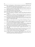
The configuration of the whole control system is outlined in Fig.1. The driver
and the motor can be modeled approximately as a second order system shown
in (84) with the system matrices
A =

01
0 −
k
fv

M

,B=

0
k
f
M

,C=

10

where M =1kg, k
fv
= 144N and k
f
=6N/V where V stands for volt. This
simple linear model does not contain any nonlinear and uncertain effects such as
the frictional force in the mechanical part, high-order electrical dynamics of the
driver, loading condition, etc., which are hard to model in practice. In general,
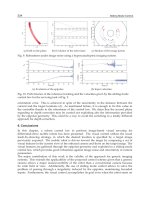
Fig. 1. System Block Diagram
262 X. Jian-Xin and K. Abidi
10
−4
10
−3
10
−2
10

−1
10
0
1
1.5
2
2.5
3
sampling−time [sec]
open−loop zero
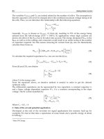
Fig. 2. Open-loop zero of (Φ, Γ, D) with respect to sampling-time
10
−4
10
−3
10
−2
10
−1
10
0
−1
−0.8
−0.6
−0.4
−0.2
0
sampling−time [sec]
open−loop zero
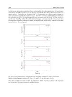
Fig. 3. Open-loop zero of (Φ, Γ, C) with respect to sampling-time

producing a high precision model will require more efforts than performing a
control task with the same level of precision.
As in all motion control problems, only position feedback is possible. Thus,
leaving us with either the output feedback approach or the state observer ap-
proach both of which we will explore separately.
6.3 Output Feedback Approach
In order for the output feedback approach to be applicable the system (Φ, Γ, D),
where D = CΦ
−1
, must be minimum phase. For discrete-time applications it is
well known that the minimum phase condition is dependent on the continuous-
time system as well as the sampling-time used. For this particular system the
plot of the open-loop zero versus the sampling-time is shown in Fig.2. It can
Output Tracking with Discrete-Time Integral Sliding Mode Control 263
0 0.2 0.4 0.6 0.8 1
0
5
10
15
20
25
30
35
40
t [sec]
y [mm]
ISMC
PI
Reference
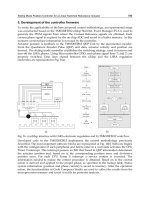
Fig. 4. Position trajectory and comparison of ISMC and PI controllers’ performance

0 0.5 1 1.5
−0.01
0
0.01
0.02
0.03
0.04
0.05
t [sec]
e [mm]
ISMC
PI
Fig. 5. Tracking error of ISMC and PI controllers
be seen that the open-loop zero approaches 1 as T →∞but is never less
than 1 which means this particular system is non-minimum phase no matter
what the sampling-time used is. Thus, this approach is inapplicable in this case,
underscoring the restrictive nature of this approach.
6.4 State Observer Approach
For the state observer approach the system (Φ, Γ, C) is required to be minimum
phase. From Fig.3 we see that for a sampling-time between 0.1ms and 1s the
open-loop zero has a relatively larger stability margin. From Fig.3 a selection of
sampling-time T =1ms would provide a fast enough convergence while having a
good enough tracking error. Upon sampling at T =1ms the resulting sampled-
data system state and gain matrices are
264 X. Jian-Xin and K. Abidi
Φ =

1.0000 0.0009
00.8659


,Γ=

2.861 ×10
−6
5.6 ×10
−3

and the open-loop zero is −0.954. To proceed with the implementation three
parameters need to be designed: the state observer gain L, the disturbance ob-
server integrator gain matrix E
d
, and the controller integrator gain E.Thestate
observer gain is selected such that the observer poles are (0.4, 0.4). This selec-
tion is to ensure quick convergence. Next, the matrix E
d
is designed. Note that
for this second order system E
d
is a scalar. To ensure the quick convergence of
the disturbance observer, E
d
is selected such that the observer pole is λ
d
=0.9
which corresponds to s = −105.4 in the continuous-time. Since the remaining
pole of the observer is the non-zero open-loop zero z = −0.954 corresponding
to a pole with real part of s = −47.1 in the continuous-time, it is the dominant
pole. Finally, the controller pole is selected as λ =0.958 which is found to be
the best possible after some trials. Thus, the design parameters are as follows
L =


1.059 231.048

,E
d
=1−λ
d
=0.1,E=1−λ =0.042.
The reference trajectory r
k
used is a sigmoid curve as shown in Fig.4. The ISM
results are compared to that of a PI controller as seen in Fig.4 and Fig.5. From
the results we see that the ISM controller has a better tracking performance
compared to a PI controller. The results in Fig.6 are for the control inputs for
the PI and ISM. Finally, an extra load of 2.5kg is added without modifying the
controller parameters. We see from the results that the change of load barely
effects the ISM controller performance as seen in Fig.7. The control for this case
is seen in Fig.8. We can observe from the figures that the control input needed
to overcome the deadzone is increased from around 1.25V to around 1.5V when
the load is added.
0 0.2 0.4 0.6 0.8 1
0
0.5
1
1.5
2
2.5
t [sec]
u [V]
ISMC

PI
Fig. 6. Comparison of the control inputs of ISMC and PI controllers
Output Tracking with Discrete-Time Integral Sliding Mode Control 265
0 0.5 1 1.5
−0.015
−0.01
−0.005
0
0.005
0.01
0.015
t [sec]
e [mm]
ISMC
Fig. 7. Position trajectory with ISMC loaded with 2.5kg
0 0.2 0.4 0.6 0.8 1
0
0.5
1
1.5
2
2.5
t [sec]
u [V]
ISMC
Fig. 8. Control input for ISMC with 2.5kg load
7Conclusion
This chapter presented a form of the discrete-time integral sliding control design
for sampled-data systems with output tracking. Three approaches are investi-
gated: 1) State Feedback, 2) Output Feedback, and 3) Output Feedback with

a State Observer. Proper disturbance and state observers were presented. The
closed-loop stability of the system was not dependent on either observer and is
designed separately. It was shown that for all the three approaches the maximum
bound on the tracking error is O(T
2
) at steady state. It was also shown that
even though the state observer produced O(T ) estimation error, the ISM state
observer approach could still produce O(T
2
) tracking error. Experimental com-
parison with a PI controller proves the effectiveness of the proposed methods.
266 X. Jian-Xin and K. Abidi
References
1.
˙
Zak, S.H., Hui, S.: On variable structure output feedback controllers for uncertain
dynamical systems. IEEE Transactions on Automatic Control 38, 1509–1512 (1993)
2. El-Khazali, R., DeCarlo, R.: Output feedback variable structure control design.
Automatica 31, 805–816 (1995)
3. Edwards, C., Spurgeon, S.K.: Robust output tracking using a sliding mode con-
troller/observer scheme. International Journal of Control 64, 967–983 (1996)
4. Slotine, J.J.E., Hedrick, J.K., Misawa, E.A.: On sliding observers for nonlinear
systems. ASME Journal of Dynamic Systems, Measurement and Control 109, 245–
252 (1987)
5. Lai, N.O., Edwards, C., Spurgeon, S.: Discrete output feedback sliding mode based
tracking control. In: Proc. 43rd IEEE Conference on Decision and Control, Nassau,
Bahamas (2004)
6. Lai, N.O., Edwards, C., Spurgeon, S.: On discrete time output feedback min-max
controller. International Journal of Control 77, 554–561 (2004)
7. Su, W.C., Drakunov, S., Ozguner, U.: An O(T

2
) boundary layer in sliding mode
for sampled-data systems. IEEE Transactions on Automatic Control 45, 482–485
(2000)
8. Utkin, V.I.: Sliding mode control in discrete-time and difference systems. In: Zi-
nober, A.S.I. (ed.) Variable Structure and Lyapunov Control. Lecture Notes on
Control and Information Sciences, vol. 193, Springer, Berlin (1994)
9. Abidi, K., Xu, J.X.: On the discrete-time integral sliding mode control. In: Proc.
IEEE Workshop on Variable Structure Systems VSS 2006, Alghero, Italy (2006)
10. Utkin, V.I., Shi, J.: Integral sliding mode in systems operating under uncertainty
conditions. In: Proc. Conference on Decision and Control CDC 1996, Kobe, Japan
(1996)
11. Cao, W.J., Xu, J.X.: Eigenvalue Assignment in Full-Order Sliding Mode Using
Integral Type Sliding Surface. IEEE Transactions on Automatic Control 49, 1355–
1360 (2004)
12. Fridman, L., Castanos, F., M’Sirdi, N., Khraef, N.: Decomposition and Robust-
ness Properties of Integral Sliding Mode Controllers. In: Proc. IEEE Workshop on
Variable Structure Systems VSS 2004, Vilanova i la Geltru, Spain (2004)
13. Astrom, K.J., Wittenmark, B.: Computer-Controller Systems. Prentice Hall, Upper
Saddle River (1997)
Appendix:ProofofLemma1
If the matrices Φ, Γ and C are partitioned as shown
Φ =

Φ
11
Φ
12
Φ
21

Φ
22

,C=

C
1
C
2

, and Γ =

Γ
1
Γ
2

where (Φ
11
,C
1
,Γ
1
) ∈
m×m
,(Φ
12
,C
2
) ∈

m×n−m
,(Φ
21
,Γ
2
) ∈
n−m×m
and
Φ
22
∈
n−m×n−m
. The eigenvalues of

Φ −Γ(CΓ)
−1
(CΦ −ΛC)

are found from
det

λI
n
− Φ + Γ (CΓ)
−1
(CΦ −ΛC)

= 0 (91)
Output Tracking with Discrete-Time Integral Sliding Mode Control 267
det

⎡
⎢
⎢
⎣
λI −Φ
11
+ Γ

1

C

Φ
11
Φ
21

− ΛC
1

−Φ
12
+ Γ

1

C

Φ
12

Φ
22

− ΛC
2

−Φ
21
+ Γ

2

C

Φ
11
Φ
21

− ΛC
1

λI −Φ
22
+ Γ

2

C


Φ
12
Φ
22

− ΛC
2

⎤
⎥
⎥
⎦
=0
(92)
where Γ

1
= Γ
1
(CΓ)
−1
and Γ

2
= Γ
2
(CΓ)
−1
. If the top row is premultiplied with
C

1
and the bottom row is premultiplied with C
2
and the results summed and
used as the new top row, using the fact that C
1
Γ
1
+ C
2
Γ
2
= CΓ the following
is obtained
det
⎡
⎣
(λI
m
− Λ)C
1
(λI
m
− Λ)C
2
−Φ
21
+ Γ

2


C

Φ
11
Φ
21

− ΛC
1

λI −Φ
22
+ Γ

2

C

Φ
12
Φ
22

− ΛC
2

⎤
⎦
=0

(93)
factoring the term (λI
m
− Λ) and premultiplying the top row with Γ
2
(CΓ)
−1
Λ
and adding to the bottom row leads to
det(λI
m
− Λ)det
⎡
⎣
C
1
C
2
−Φ
21
+ Γ

2
C

Φ
11
Φ
21


λI
n−m
− Φ
22
+ Γ

2
C

Φ
12
Φ
22

⎤
⎦
=0. (94)
Thus, we can conclude that m eigenvalues of

Φ −Γ(CΓ)
−1
(CΦ −ΛC)

are the
eigenvalues of Λ.Now,consider
det
⎡
⎣
C
1

C
2
−Φ
21
+ Γ

2
C

Φ
11
Φ
21

λI
n−m
− Φ
22
+ Γ

2
C

Φ
12
Φ
22

⎤
⎦

=0. (95)
Using the following relations
C
2
Φ
21
− C
2
Γ

2
C

Φ
11
Φ
21

= −C
1
Φ
11
+ C
1
Γ

1
C

Φ

11
Φ
21

(96)
C
2
Φ
22
− C
2
Γ

2
C

Φ
12
Φ
22

= −C
1
Φ
12
+ C
1
Γ

1

C

Φ
12
Φ
22

, (97)
and multiplying (95) with λ
−m
λ
m
we obtain
λ
−m
det
⎡
⎣
λC
1
λC
2
−Φ
21
+ Γ

2
C

Φ

11
Φ
21

λI
n−m
− Φ
22
+ Γ

2
C

Φ
12
Φ
22

⎤
⎦
=0. (98)
Premultiplying the bottom row with C
2
and subtracting from the top row and
using the result as the new top row we have
λ
−m
det
⎡
⎢

⎢
⎣
λC
1
+ C
2
Φ
21
− C
2
Γ

2
C

Φ
11
Φ
21

C
2
Φ
22
− C
2
Γ

2
C


Φ
12
Φ
22

−Φ
21
+ Γ

2
C

Φ
11
Φ
21

λI
n−m
− Φ
22
+ Γ

2
C

Φ
12
Φ

22

⎤
⎥
⎥
⎦
=0.
(99)
268 X. Jian-Xin and K. Abidi
Using relations (96) and (97) we finally obtain
λ
−m
det
⎡
⎢
⎢
⎣
λC
1
− C
1
Φ
11
+ C
1
Γ

1
C


Φ
11
Φ
21

−C
1
Φ
12
+ C
1
Γ

1
C

Φ
12
Φ
22

−Φ
21
+ Γ

2
C

Φ
11

Φ
21

λI
n−m
− Φ
22
+ Γ

2
C

Φ
12
Φ
22

⎤
⎥
⎥
⎦
=0.
(100)
We can factor out the matrix C
1
from the top row to obtain
λ
−m
det(C
1

)det
⎡
⎢
⎢
⎣
λI
m
− Φ
11
+ Γ

1
C

Φ
11
Φ
21

−Φ
12
+ Γ

1
C

Φ
12
Φ
22


−Φ
21
+ Γ

2
C

Φ
11
Φ
21

λI
n−m
− Φ
22
+ Γ

2
C

Φ
12
Φ
22

⎤
⎥
⎥

⎦
=0
(101)
which finally simplifies to
λ
−m
det(C
1
)det[λI + Φ − Γ (CΓ)CΦ]=0. (102)
It is well known that [Φ − Γ (CΓ)CΦ] has at least m zero eigenvalues which would
be canceled out by λ
−m
and, thus, we finally conclude that the eigenvalues of

Φ − Γ (CΓ)
−1
(CΦ −ΛC)

are the eigenvalues of Λ and the non-zero eigenvalues
of [Φ − Γ (CΓ)CΦ].