Road Traffic Noise Shielding by Vegetation Belts of Limited Depth

Road traffic noise shielding by vegetation belts of limited depth
T. Van Renterghem
a,
n
, D. Botteldooren
1,a
, K. Verheyen
2,b
a
Ghent University, Department of Information Technology, Sint-Pietersnieuwstraat 41, B-9000 Gent, Belgium
b
Ghent University, Department of Forest and Water Management, Geraardsbergsesteenweg 267, B-9090 Melle-Gontrode, Belgium
article info
Article history:
Received 25 May 2011
Received in revised form
12 December 2011
Accepted 9 January 2012
Handling Editor: J. Astley
Available online 7 February 2012
abstract
Road traffic noise propagation through a vegetation belt of limited depth (15 m)
containing periodically arranged trees along a road is numerically assessed by means
of 3D finite-difference time-domain (FDTD) calculations. The computational cost is
reduced by only modeling a representative strip of the planting scheme and assuming
periodic extension by applying mirror planes. With increasing tree stem diameter and
decreasing spacin g, traffic noise insertion loss is predicted to be more pronounced
for each planting scheme considered (simple cubic, rectangular, triangular and
face-centered cubic). For rectangular schemes, the spacing parallel to the road axis is
predicted to be the determining parameter for the acoustic performance. Significant
noise reduction is predicted to occur for a tree spacing of less than 3 m and a tree stem

diameter of more than 0.11 m. This positive effect comes on top of the increase in
ground effect (near 3 dBA for a light vehicle at 70 km/h) when compared to sound
propagation over grassland. The noise reducing effect of the forest floor and the
optimized tree belt arrangement are found to be of similar importance in the
calculations performed. The effect of shrubs with typical above-g round biomass is
estimated to be at maximum 2 dBA in the uniform scattering approach applied for a
light vehicle at 70 km/h. Downward scattering from tree crowns is predicted to be
smaller than 1 dBA for a light vehicle at 70 km/h, for various distribu tions of scattering
elements representing the tree crown. The effect of the presence of tree stems, shrubs
and tree crowns is predicted to be approximately additive. Inducing some (pseudo)
randomness in stem center location, tree diameter, and omitting a limited number of
rows with trees seem to hardly affect the insertion loss. These predictions suggest that
practically achievable vegetation belts can compete to the noise reducing performance
of a classical thin noise barrier (on grassland) with a height of 1–1.5 m (in a non-
refracting atmosphere).
& 2012 Elsevier Ltd. All rights reserved.
1. Introduction
The acoustical effect of a belt of trees/vegetation near roads has been a popular research topic over the past 40 years
[1–10]. The conclusions drawn from such experiments are, however, often quite different. Aylor looked at sound
propagation through corn, a hemlock plantation, a pine stand, and hardwood brush [1], and over dense reeds above a
Contents lists available at SciVerse ScienceDirect
journal homepage: www.elsevier.com/locate/jsvi
Journal of Sound and Vibration
0022-460X/$ - see front matter & 2012 Elsevier Ltd. All rights reserved.
doi:10.1016/j.jsv.2012.01.006
n
Corresponding author. Tel.: þ32 9 264 36 34; fax: þ32 9 264 99 69.
E-mail addresses: (T. Van Renterghem), (D. Botteldooren),
(K. Verheyen).
1

Tel.: þ32 9 264 99 68; fax: þ32 9 264 99 69.
2
Tel.: þ32 9 264 90 27; fax: þ32 9 264 90 92.
Journal of Sound and Vibration 331 (2012) 2404–2425
water surface [2]. He concluded that the leaf area density should be high, and leaves should be broad and thick to see
significant effects. Visibility was considered to be a bad predictor of the attenuation capacity of a vegetative stand [1].
Thirty-five tree belts were studied by Fang and Ling [7]. Multiple linear regression analysis on their data showed that
visibility through the vegetation and the width of the belt were the major parameters. Other parameters contributing to an
improved prediction were height and length of the belt. The typical leaf size at the tested locations was considered to be
rather unimportant in their regression model. Tyagi et al. [9], on the other hand, linked the significantly higher attenuation
at the 3.15-kHz 1/3-octave band to the dimensions of the plant structures in their measurements. Pathak et al. [10]
measured that belt width and tree height are positively correlated with traffic noise reduction. Pal et al. [6] measured near
12 vegetation belts and found that the average density and height of the plants has only a very small effect. Larger plant
heights could even be negative, probably due to increased downward scattering towards receivers. Vertical and horizontal
light penetration were found to be major parameters. Kragh [4] stated that the traffic noise reduction obtained by a belt of
vegetation is rather limited. In his study, sound propagation through belts of vegetation was compared to sound
propagation over grassland over the same distance. Significant attenuation was provided by the vegetation only above
2 kHz.
In many of the above mentioned publications, the reference situation when assessing the effect of the vegetation belts
is rather unclear. Furthermore, many effects related to the interaction between sound and vegetation were jointly
observed. This makes it difficult to derive design rules for vegetation belts. In this paper, numerical calculations are used to
assess the effect of vegetation belts of limited width along roads. In contrast to in-situ measurements, the reference
situation can be well defined and the various effects can easily be separated out. On the other hand, modeling approaches
always induce some idealizations.
Basically, vegetation is able to reduce sound levels in three ways. First, sound can be reflected and scattered (diffracted)
by plant elements like trunks, branches, twigs and leaves. Very close to vegetation and below tree crowns, this could lead
to increased sound levels by downward scattering [11]. In many applications, however, sound energy will leave the
line-of-sight between source and receiver when interacting with vegetation, leading to reduced sound pressure levels.
A second mechanism is absorption caused by vegetation. This effect can be attributed to mechanical vibrations of plant
elements caused by sound waves [12–14] which lead to dissipation by converting sound energy to heat. There is also a

contribution to attenuation by thermo-viscous boundary layer effects at vegetation surfaces. As a third mechanism, one
might also mention that sound levels can be reduced by destructive interference of sound waves. The presence of the soil
can lead to destructive interference between the direct contribution from source to receiver, and a ground-reflected
contribution. This effect is often referred to as the acoustical ground effect or ground dip. The presence of vegetation leads
to an acoustically very soft (porous) soil, mainly by the presence of a litter layer and by plant rooting. This results in a more
pronounced ground effect and in a shift towards lower frequencies compared to sound propagation over grassland [15].
As a result, this ground dip is more efficient in limiting typical engine noise frequencies (near 100 Hz) of road traffic.
Besides these direct acoustical effects, some indirect effects can be mentioned as well. Forests change the refractive
state of the lower part of the atmosphere and therefore influence sound propagation as studied, e.g. in [15–18]. Near a
noise barrier, a row of trees was shown to limit the screen-induced refraction of sound by the action of the wind [19,20],
and the specific distribution of biomass in the canopy plays a role [21]. Fricke [22] measured that sound attenuation is
influenced to an important degree by the relative humidity inside a forest, in a way that cannot be explained by the action
of atmospheric absorption or by changes in soil humidity. Another type of indirect effects deals with psycho-acoustical
effects. Wind-induced vegetation noise can lead to masking of unwanted sounds, and as a result, there has been interest in
predicting this effect [23,24]. Traffic noise perception is also influenced by visual stimuli: with an increasing degree of
urbanization (and as a result less vegetation), the perception becomes less pleasant [25].
In periodic structures, so-called acoustic band gap effects might appear (see e.g. Refs. [26,27]): Waves scattered by the
components of a lattice (or the elements with a sufficient contrast in density relative to the propagation medium)
interfere. This could lead to large noise reductions in particular frequency bands. The spacing between the scattering
elements (lattice constant) determines the stop-band central frequencies, the filling fraction their efficiency. Applications
and research mainly focus on closely packed cylinders [26–28]. An interesting question is whether such effects can be
achieved by introducing periodicity in vegetation belts, keeping in mind realistic plant densities. The latter imply that the
maximum filling fractions are limited. However, experiments with trees organized in periodic arrays were also found to
produce attenuation peaks at frequencies below 500 Hz due to band gap effects, and not as a consequence of interaction
with the ground surface as was discussed in Ref. [29]. Total traffic noise shielding was not assessed in this earlier work.
Numerical calculations with relation to sound propagation through belts of vegetation or forests all start from random
orderings. In Ref. [30], tree stems were explicitly modeled in 3D with a FDTD model. In Refs. [16,18
,31], multiple scattering
theory for randomly spaced arrays of cylinders was used to predict sound propagation through forests.
Given the findings in recent sonic crystal research and taking into account the work reported in Ref. [29], studying

periodic plant organizations seems worth the effort. Periodic planting schemes are also beneficial as regards the
computational cost. 3D numerical simulations typically need a very large amount of computational resources. However,
as a result of exploiting periodicity, the computational domain can be largely reduced. This is done by using mirror planes
in the simulation domain, and only modeling a representative strip of the grid. Making advantage of symmetry is a sound
approach in acoustical simulations, and applications of this concept are numerous. Applications of the mirror plane
approach to 3D time-domain outdoor sound propagation calculations can be found, e.g. in Refs. [32,33].
T. Van Renterghem et al. / Journal of Sound and Vibration 331 (2012) 2404–2425 2405
A drawback of the mirror plane approach in the current context is that only planting schemes that are periodic in a
direction parallel to the road axis can be modeled. From sonic crystal research, it was shown, e.g. that some defects in the
lattice could be beneficial to broaden the frequency range where sound reduction is observed [34]. Orthogonal to the road
axis, such effects could be included and will be studied.
As illustrated by the references in the previous paragraphs, the typical ground under vegetation could be a major effect
in reducing noise. So the positive effect of the ground should preferably be preserved, and its interaction with the multiple
scattering between vegetation elements should be studied. The interaction between the soil effect and the presence of
scattering vegetation is not always clear when looking at literature. In Ref. [1], it was written that adding the separate
effects of leaves, stems and ground to obtain the total effect for any combination of these is not unreasonable. The
measurements performed in Ref. [31] lead to similar conclusions. In Ref. [15], on the other hand, it was stated that this
interaction is more complicated than simply additive. Bullen and Fricke [35] found that that the largest effects of placing
cylinders in their scale model of a strip of vegetation were observed above a rigid plane and for a sound frequency of 4 kHz.
For an acoustically absorbing ground, the insertion loss (IL) relative to the same type of ground cover in absence of
cylinders was much more moderate. Krynkin and Umnova [36] found that in their calculations of a sonic crystal made of
rigid cylinders (with their axes parallel to the ground surface), the largest IL values were found for sound propagation over
a rigid ground. The 3D calculations performed in this study will contribute to this discussion.
In this paper, planting schemes on a typical soil as found under vegetation, in a 15-m wide belt bordering a road, are
numerically assessed. Focus is on total road traffic noise levels of light vehicles. The maximum frequency considered in this
study (the 1.6-kHz one-third octave band) takes into account a relevant part of the tire/road interaction noise, and allows a
more complete estimation of possible traffic noise reduction than in the related study of Heimann [30] where the
maximum sound frequency that could be attained was 600 Hz.
Note that some of the modeled configurations have a tree density that would be very hard to realize in practice.
However, such simulations could be helpful to reveal trends. Practical aspects will be discussed and it is indicated what

configurations could be realized. Also, results will be compared to sound propagation over a grass-covered land with
identical source–receiver configuration. This allows policy makers and urban planners to get a global and quantitative idea
of the gain obtained by changing a piece of grassland into a tree/vegetation belt. Given the rather short propagation
distance between source and receiver, refraction effects will be very limited and will not be considered here.
In addition, a simple scattering model is proposed to assess the effect of small ground-covering vegetation, shrubs, and
tree crowns. One has to keep in mind that scattering by vegetation is mainly a high-frequency phenomenon since most
structures in, e.g. a tree crown are very small compared to the dominant wavelengths in a road traffic noise spectrum.
Furthermore, the density of the scatterers (volume fraction) is limited. Martens [37], e.g. stated that scattering by
vegetation is rather unimportant when looking at total traffic noise level reduction. Measurements behind a noise barrier
with and without the presence of a row of trees in Ref. [19] showed that scattering by the trees can be significant at very
high frequencies (þ5 dB at 10 kHz). At the 1.6 kHz one-third octave band, which will be the maximum frequency
considered in this study, the amount of scattering was only near þ1 dB. As a result, most important effects are expected
from the presence of stems of trees (in combination with soil as appears under vegetation) which is the main concern in
this paper. However, including these additional effects allows for a more complete assessment of the noise reducing effects
of vegetation belts.
This paper is organized as follows. The FDTD model is briefly described in Section 2. In the next section, the choice of
the simulation parameters is discussed. In Section 4, the scattering approach is presented, for the case of sound
propagation through shrub layers and for tree crown scattering. In Section 5, 3D –FDTD calculation results are presented
for road traffic noise shielding by vegetation belts of limited depth. In Section 6, some practical considerations concerning
the feasibility of the modeled tree stands are made. In Section 7, conclusions are drawn. In the appendices, approaches
aiming at reducing the computational cost are checked, and a summary of all simulations performed in this study is
presented.
2. The finite-difference time-domain model
The following equations describe sound propagation in air:
=
Upþ
r
0
@v
@t

¼ 0, (1)
@p
@t
þ
r
0
c
0
2
=
Uv ¼ 0: (2)
In the linear Eqs. (1) and (2), p is the acoustic pressure, v is the particle velocity,
r
0
is the mass density of air, c
0
is the
adiabatic sound speed, and t denotes time. A homogeneous and still propagation medium is assumed. Viscosity, thermal
conductivity, molecular relaxation, and gravity are neglected.
T. Van Renterghem et al. / Journal of Sound and Vibration 331 (2012) 2404–24252406
The interaction between sound waves and the soil in this study is simulated by means of the Zwikker and Kosten
phenomenological model [38]:
=
Upþ
r
0
k
s
j
@v

@t
þRv ¼0, (3)
@p
@t
þ
r
0
j
c
0
2
k
s
=
Uv ¼ 0, (4)
In Eqs. (3) and (4), R is the flow resistivity of the porous medium,
j
its porosity and k
s
the structure factor. These
equations describe sound propagation in a porous rigid-frame medium.
The finite-difference time-domain (FDTD) method is used to solve Eqs. (1)–(4). The efficient staggered-in-time and
staggered-in-space discretisation approach is chosen [39]. The advantages of this numerical scheme were described
elsewhere [39]. Implementing the Zwikker and Kosten model does not induce additional difficulties compared to Eqs. (1)
and (2) [20,40]. The validity of this model to simulate the interaction between sound waves and different types of outdoor
soils has been discussed in Ref. [41].
Rigid surfaces are easily modeled by setting the normal component of the particle velocity to zero. Tree barks are
modeled as a frequency-independent real-valued surface impedance as shown in [42]. The validity of this simplification is
discussed in Section 3.4.
The FDTD method has been validated by comparison with measurements, analytical solutions and other numerical

methods, over a wide range of acoustical applications [43,20,44,45].
3. Simulation parameters
3.1. Basic FDTD parameters
The spatial discretisation step is chosen to be 0.02 m, which is a compromise between limiting the computational cost
and sufficiently capturing the road traffic noise frequency range. This means that calculations can be performed up to
1700 Hz (with a sound speed of 340 m/s), when demanding that at least 10 computational cells per wavelength are needed
for accuracy reasons. A staggered, cubic spatial discretisation grid is used. The temporal discretisation step is taken so that
the Courant number equals 1, leading to minimal phase errors, numerical stability and minimum computing times [39].
3.2. Simulation setup
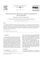
An overview of the grid setup with dimensions is shown in Fig. 1. A line source at a height of 0.3 m (typical engine noise
source height for light vehicles following the Harmonoise/Imagine road traffic source power model [46]) is placed above a
rigid plane. A rigid plane is representative for a road surface top layer like concrete. Sound propagation in the soil layer
itself (with a thickness of 0.5 m) is included in the simulation domain. A receiver plane is placed at 19 m from the source.
A zone of 15 m in between the source and the receiver plane will be used to investigate the effect of various planting
schemes. Perfectly matched layers are used to simulate an unbounded atmosphere at the left, right and upper boundary.
Rigid planes are applied at x¼0 and w
rs
to model periodic extension of both the line source and the planting scheme
considered. The width of the representative strip w
rs
that is modeled depends on the chosen planting scheme, and is at
Fig. 1. Basic 3D grid setup ((a) cross-section and (b) plan view), showing the zone reserved for the evaluation of a specific planting scheme, the location
of the line source and receiver plane, and the location of the perfectly matched layers (PML). The distance between the two mirror planes is indicted by
w
rs
and depends on the planting scheme.
T. Van Renterghem et al. / Journal of Sound and Vibration 331 (2012) 2404–2425 2407
minimum 1 m and at maximum 3 m. The validity of the mirror plane approach is checked by the 2D numerical example in
Appendix A.
3.3. Soil parameters

In Ref. [41], reasonably accurate fits to measurements were found using the Zwikker and Kosten phenomenological
model in case of sound propagation over forest floor and over grass-covered land. For these types of soil, very similar errors
were found when using the slit-pore frequency-impedance model. For grass-covered ground, 26 sites were considered in
Ref [41], ranging from ‘‘lawns’’ to ‘‘pastures’’. Based on these data, an (effective) flow resistivity of 300 kPa s m
À2
and a
porosity of 0.75 have been used to represent grassland in the current calculations. Measurements of the ground effect at
pine stands and beech forests were considered as well in Ref. [41]. A flow resistivity of 20 kPa s m
À2
and a porosity of 0.5
have been used to simulate the soil appearing under vegetation. The relation between porosity and tortuosity as described
in Ref. [41] is applied.
Note that the main interest in these simulations is modeling reflection from a typical soil as found under vegetation.
When there is interest in predicting the attenuation inside the porous medium itself, for the specific case of high sound
frequencies and low flow resistivities, adaptations to the Zwikker and Kosten model should be made as proposed, e.g. in
Ref. [47].
In this numerical study, the influence of a specific tree stand (tree species, tree spacing, presence of shrubs, etc.) on soil
properties is not considered.
3.4. Acoustical properties of tree bark
Sound absorption of tree bark was studied by Reethof et al. [42] in an impedance tube (normal incident sound waves).
Samples of the bark of species like Quercus, Tsuga, Pinus, Fagus, and Carya were considered. The absorption coefficients
were mainly between 0.05 and 0.10 for sound frequencies between 400 Hz and 1600 Hz. For most species, effects were
rather frequency independent in this range. Some species like Carya (Mockernut) gave significant higher absorption values,
ranging up to 0.25 at 1.6 kHz. Based on these findings, an average frequency-independent value of 0.075 (normal
incidence) can be justified for modeling reflection on the tree barks. This leads to a real-valued impedance of 51 times the
impedance of air.
3.5. Planting schemes
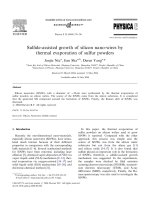
In this study, four different tree planting schemes are considered, namely a simple cubic scheme (SC), a simple
rectangular (SR) scheme, a face-centered cubic scheme (FCC) and a triangular scheme (T). The basic parameter to represent
a certain scheme is the minimum distance between adjacent tree stem axes. This minimum distance is indicated by d in

the SC, FCC and T scheme, and by d
1
(parallel to the road axis) and d
2
(normal to the road axis) in the SR scheme. In this
representation, the SC and FCC have the same tree density per unit area (¼1/d
2
), while the planting scheme T is somewhat
more dense (factor 2=
ffiffiffi
3
p
). The SR schemes have a tree density of 1/(d
1
d
2
).
In Fig. 2, a representative strip is shown for each grid element. In case of a SC or SR scheme, such a strip is symmetric.
In case of a FCC and T scheme, the computational cost can be further reduced by considering an asymmetric strip, cutting
the stems at the borders in two.
Fig. 2. Simple cubic (SC, d
1
¼d
2
¼d) (a), simple rectangular (SR, characterized by d
1
and d
2
) (a), face-centered cubic (characterized by its minimum
distance d between stems) (b), and triangular scheme (characterized by its minimum distance d between stems) (c). The representative strip is bordered

by the dashed rectangles.
T. Van Renterghem et al. / Journal of Sound and Vibration 331 (2012) 2404–24252408
4. Approximation for small scattering elements
Explicitly modeling each element in vegetation imposes difficulties, especially in a volume discretisation technique
employing a uniform grid as FDTD. The smallest structure that can be easily modeled is the computational cell.
A meaningful representation of a small twig is usually not possible in a 3D grid without using techniques as grid
refinement, conformal grids or subgrid-scale modeling which in all cases leads to more complex calculation schemes and a
higher computational cost. A valuable approach is subgrid-scale modeling [48], as illustrated by means of the pseudo-
spectral time-domain (PSTD) model where scattering was modeled near a small tree based on a detailed geometrical
representation of it [49]. A main problem with using full geometrical details is access to such data, and the loss of the
naturally occurring variation in such structures. Therefore, a more practical and easy-to-apply approach is proposed here.
It is based on a statistical spatial distribution of (basic) filled grid cells, imitating the interaction between vegetation
structures and sound waves, while preserving the inherent randomness. Besides modeling of multiple scattering and a
high portion of transmission through the vegetation, the effect of absorption by branches and twigs can be included by
making these filled cells partly absorbing. Focus is on scattering by woody material. Important interactions between leafs
and sound waves are expected to occur at sound frequencies beyond the range that is modeled here [19], and is considered
to be of limited importance when looking at total A-weighted road traffic noise [37].
4.1. Low growing vegetation and shrubs
Firstly, this approach will be used to model the interaction between sound and shrubs and other low, ground-covering
vegetation. Near full ground cover is possible for many species or combinations of species. As a result, a uniform
distribution of scatterers will be assumed. The above-ground woody biomass volume taken by the shrubs is then evenly
distributed over the artificial scatterering cells in FDTD. Given the absence of more detailed data on the acoustic surface
properties of the branches and twigs for this type of vegetation, the same data as for tree bark is used (see Section 3.4).
The addition of (some) absorption will not only account for the interaction between the surface of plant material and
acoustic waves, but also for damping by sound-induced vibration of plant elements.
For the FDTD calculations, the input parameter in the above described approach is 1 minus the porosity of the shrubs,
which equals the chance of making a grid cell a scattering cell. Information on this parameter is not directly available in
relevant literature. The basic parameter that is found is the above-ground total dry biomass per unit area. In combination
with typical shrub height, mass distribution over leafs and woody parts, mass density of dry wood in shrubs, and the
typical water content of woody parts, the above-ground shrub porosity can be estimated.

A wide range of values for above-ground (oven-dried) total biomass per unit area can be found in literature.
The measurements in Ref. [50] for different shrub type ecosystems reported values from 0.5 to 2 kg/m
2
, for shrubs heights
lower than 1.5 m and ground coverage ranging from 42 percent to 97 percent. Furthermore, an overview is given in [50]
for some Mediterranean species, showing values in the range from 1 kg/m
2
to 6.68 kg/m
2
, for shrub heights ranging
from 1 m to 4.5 m. The average value for low trees and shrubs (12 species) reported by Harrington [51] was 5.4 kg/m
2
.
Navar et al. [52] found an average of above-ground total biomass per unit area of 4.44 kg/m
2
. Top heights of the various
species involved in the latter ranged from 1.9 m to 5 m.
The distribution of biomass over leafs, branches and stems was measured to be 5.6 percent, 61.5 percent, and 32.8
percent, respectively, in Ref. [52]. Measured values for the ratio leafs to total above-ground biomass ranged between 3
percent and 34 percent, with a median at 18 percent as reported in Ref. [51]. Navarro-Cerrillo and Blanco-Oyonarte [50]
give an overview of photosynthetic-to-total phytomass values for many species; most of the data fell in the range between
12 percent and 19 percent.
The water content and water distribution between woody biomass and leafs depend on many variables like plant
segment, stand location, age, etc. [53]. The water content in the woody parts was found to be typically 40 percent
according to the measurements in [53]. This is consistent with the typical range of water content of leafs in deciduous
shrubs ranging from 50 percent (older full-size leafs) to 65 percent (lush new leafs) according to Ref. [54]. In Ref. [53],
measurements showed values between 50 percent and 60 percent.
Mass density of (dry) wood in shrubs falls in the range from 400 to 1100 kg/m
3
[55]. These values depend largely on

shrub species. The median value on this data is close to 650 kg/m
3
.
The in-situ shrub porosity
j
shrubs
of woody plant elements can then be calculated as follows:
j
shrubs
¼ 1À
m
tot, dry
H
shrubs
f
wood, dry
r
wood, dry
þ
f
wood, dry
r
water
w
wood
1Àw
wood

"#
, (5)

with m
tot,dry
the total, dry above-ground biomass (in kg/m
2
), H
shrubs
the average height of the shrubs (in m), f
wood,dry
the
mass fraction taken by the dry wood,
r
wood,dry
the mass density of dry wood (in kg/m
3
),
r
water
the mass density of water,
and w
wood
the fraction of water present in woody parts of the shrubs in-situ. When using typical values from the literature
review as discussed above (m
tot,dry
¼4 kg/m
2
, f
wood,dry
¼0.9,
r
wood,dry

¼650 kg/m
3
,
r
water
¼1000 kg/m
3
, w
wood
¼0.4) and by
taking H
shrubs
¼1 m, this leads to an in-situ shrub porosity of near 0.99, meaning that 1 percent of the volume is taken
in-situ by water-containing woody plant material. Values of 0.98 and 0.995 are modeled as well to study the range of
T. Van Renterghem et al. / Journal of Sound and Vibration 331 (2012) 2404–2425 2409
possible effects given the use of default values only. Note that such values could be representative for many combinations
of the above described parameters.
4.2. Scattering from tree crowns
Including tree crowns is mainly intended to estimate the negative effect of downward scattering in the simulations.
The tree crown is – in a first approximation – represented by a sphere. The upper half of this sphere is neglected to limit
the computational domain in the y-direction. The use of small, scattering elements is applied here as well. It is assumed
that near the center of the crown, most woody material is present leading to a higher chance of filling a given
computational cell. Such a larger chance will lead to clustering of filled grid cells, which could be representative for bigger
structures in the crown like a prolongation of the stem, or bigger branches. At the surface of the sphere representing the
tree crown, a very small change that a grid cell becomes a scattering cell is applied. Note that since the frequency content
in the current simulations is limited to 1700 Hz, effects by the presence of leafs will be rather limited and this effect is
neglected. Since the exact distribution of biomass in a tree crown is not known, various approaches were tested as regards
the distribution of scattering elements to have an idea on the sensitivity of the conclusions on such choices.
5. 3D numerical calculations
The 3D numerical results are depicted in different ways in the remainder of this paper. In a first representation, (total)

traffic noise insertion loss values (in dBA) are linearly averaged over all receivers in the plane at z¼19 m and shown by
means of bar plots. A light vehicle (vehicle type 1 following the Harmonoise/Imagine road traffic source model,
representative for a passenger car) at a vehicle speed of 70 km/h is modeled. Separate bars are shown for receiver heights
ranging from ground level up to 3 m, and for receiver heights from 1 to 2 m (height of human ear for both children and
adults). Averaging over a range of receivers summarizes results. As a reference, the same type of ground has been used
(although hypothetical, the typical soft ground only develops under vegetation). In this way, the effect of the ground is
singled out, and the effect of the presence of the stems and vegetation only is assessed. An alternative reference situation is
sound propagation over grassland. As discussed in Section 1, these results give a global estimate of what can be expected
when replacing an existing piece of grassland by a vegetation belt. Furthermore, insertion loss spectra are shown at a
single receiver height along the representative strip, or as (linearly) averaged results over the receiver plane in function of
vehicle speed in case of a more detailed analysis.
A single source at a height of 0.3 m is considered (following the Harmonoise/Imagine road traffic source model), and
both the engine and rolling noise source power is assigned to that source height. The effect of also considering sound
propagation from a source at a height of 0.01 m, relative to the road surface, was shown to be limited in the current setup
and averaging approach (see Appendix B). Unless otherwise stated, the stems have a length of 2.5 m, stem diameters are
constant in the tree belt, and the full area assigned for vegetation as shown in Fig. 1 is used. The acoustic effects of the
various layers in the vegetation belt (shrub zone, stem zone, and crown zone) are considered separately to study their
individual effect, unless stated otherwise. Furthermore, a coherent line source is modeled. In Appendix C, the effect of
source type (coherent versus incoherent line source) is studied for some configurations. An overview of the 3D simulations
performed can be found in Tables D1 and D2 in Appendix D.
5.1. Effect of soil
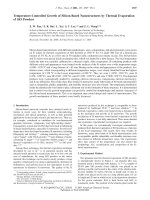
The effect of the presence of a typical soil as found under vegetation is compared to sound propagation over grassland,
for total traffic noise (light vehicles) at different vehicle speeds in Fig. 3. With increasing height above the ground surface,
the effect of a different soil becomes less pronounced. Traffic noise insertion losses at low vehicle speeds are dominated by
0 2 4 6 8 10
0
0.5
1
1.5
2

2.5
3
traffic noise IL (dBA)
Height (m)
0 2 4 6 8 10
0
0.5
1
1.5
2
2.5
3
traffic noise IL (dBA)
Height (m)
0 2 4 6 8 10
0
0.5
1
1.5
2
2.5
3
traffic noise IL (dBA)
Height (m)
rel. grass
rel. rigid
Fig. 3. Traffic noise insertion loss with height for various vehicle speeds ((a) 30 km/h, (b) 70 km/h, and (c) 110 km/h), in case of sound propagation over
uncovered vegetation soil. Results are referenced to sound propagation over grass-covered and rigid ground.
T. Van Renterghem et al. / Journal of Sound and Vibration 331 (2012) 2404–24252410
low frequencies and lead to less variation with height. Measurements of sound propagating over acoustically soft ground

from a source at limited height show similar behavior [56]. Close to the ground, differences between the two types of soils
at the higher vehicle speeds may exceed 7 dBA. The average effect for a vehicle speed of 70 km/h equals 3.3 dBA (with a
standard deviation of 1.2 dBA) for receivers between y¼0 m and 3 m, and 3.2 dBA (standard deviation of 0.5 dBA) for
receivers between y¼1 m and 2 m. For comparison, results are also referenced to sound propagation over a rigid ground in
Fig. 3, showing a large decrease in traffic noise insertion loss.
5.2. Analysis of band gap effects
In this section, the presence of band gap effects is examined for both 2D and 3D calculations for the SR 1 m/2 m scheme,
for cylinders/tree stems with diameters of 22 and 44 cm. In the first case, a coherent plane wave and infinitely long
cylinders are modeled in absence of a ground plane (and referenced to free field sound propagation). In the second case,
a coherent line source is modeled and 2.5 m-high stems above an absorbing ground (and referenced to sound propagation
over the same ground in absence of stems). Both fully rigid stems and partly absorbing stems are considered. Results are
represented as 1/9 octave bands to have a more detailed look at the insertion loss spectrum. For each receiver position, the
insertion loss is calculated. Next, the insertion losses over all receiver positions are linearly averaged. A receiver height of
2 m is considered in case of the 3D simulations.
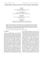
The lowest-order insertion loss peaks at 85 Hz and 170 Hz in Figs. 4 and 5 correspond to interference of scattered waves
for inter-stems distances of 2 m normal to the road (for a speed of sound equal to 340 m/s). These peaks correspond to
Bragg’s law for normal incident waves. It can be observed that such peaks are more pronounced for plane wave sound
propagation than for sound propagation over an absorbing ground surface, which is consistent with findings in [36].
At these low frequencies, only the 44-cm diameter stems provide a sufficient amount of scattering. For the 22-cm diameter
stems, only a very small insertion loss is observed at these same frequencies. For the latter, higher order band gaps will
make the more important contributions to overall IL. Modeling an incoherent line source does not seem to affect the
frequency and magnitude of these peaks (not shown). Further analysis confirms that mainly the spacing normal to
the road determines at what frequencies insertion loss peaks are found. On the other hand, decreasing the spacing along
the road increases the magnitude of the insertion loss peaks due to the increased filling fraction. A sufficient amount of
back scattering is needed, given the limited depth of the vegetation area considered. As an example, a SR 2 m/3 m 44 cm
gives similar low-frequency insertion loss peaks as SR 1 m/3 m 44 cm (easy-to-identify peaks are situated at 57 Hz, 113 Hz,
170 Hz, 227 Hz), but the magnitude of these is more pronounced with a spacing along the road of 1 m (not shown).
At higher frequencies, both interference corresponding to higher-order harmonics of the basic lattice spacing, and
direct shielding by the tree stems is observed, yielding complex insertion loss spectra. At very low frequencies, uniformity
over the modeled strip is observed. At higher frequencies, on the other hand, there is significantly more variation in

insertion loss along the representative strip, clearly shown by the larger values for the standard deviation: The exact
location relative to the position of the stems plays a more important role.
Including the absorption characteristics of tree bark seems to broaden the low-frequency peaks to a limited extent.
At higher frequencies, including absorption increases the insertion loss relative to the rigid stems, although frequency
independent impedances are modeled at the surfaces. While the 2D insertion loss values are positive over the full
10
2
10
3
0
5
10
15
20
25
30
Frequency (Hz)
IL (dB)
2D SR 1m/2m 44cm rigid
2D SR 1m/2m 22cm rigid
2D SR 1m/2m 44cm abs
2D SR 1m/2m 22cm abs
Fig. 4. Plane wave IL spectra for SR 1 m/2 m schemes, averaged over the width of the representative strip, for stem diameters of 22 cm and 44 cm, and for
rigid and partly absorbing stems. The error bars have a total length of two times the standard deviation. The reference is free field sound propagation.
T. Van Renterghem et al. / Journal of Sound and Vibration 331 (2012) 2404–2425 2411
frequency range considered, an increase in the sound level is observed near 300 Hz for the 3D case and rigid stems.
Such negative effects are somewhat less pronounced when applying typical absorption values for tree bark.
It can be concluded that the presence of the typical soil appearing under vegetation, or source representation (coherent
line source, incoherent line source, or plane wave) does not affect the possibility to exploit periodicity. Tackling engine
noise (near 100 Hz) by using the periodicity in tree belts seems difficult. Large stem diameters are needed to yield a

sufficient amount of scattered energy at these low frequencies. Furthermore, this condition is enhanced since in case of a
larger spacing a sufficient filling fraction still has to be obtained. For practical combinations of tree stem diameter and tree
spacing (see discussion in Section 6), pronounced band gap effects will therefore be mainly expected in case of limited
spacings (e.g. SC 1 m 11 cm), so at frequencies where we can also expect direct shielding effects.
5.3. Effect of stem diameter and planting scheme
The effect of the tree diameter and the choice of the planting scheme become clear from Fig. 6. Three stem diameters
were considered, namely 11 cm, 22 cm, and 44 cm, and for a passenger car at a vehicle speed of 70 km/h. The simulation
results at vehicle speeds of 30 km/h and 110 km/h can be found in Table D1. Many of the planting schemes with the 44 cm
tree diameters, and some of the 22 cm tree diameters, will be hard to achieve in practice, but were retained as they allow a
better evaluation of the importance of some parameters. Remarks on practical aspects can be found in Section 6.
With increasing tree stem diameter, traffic noise insertion loss is more pronounced for each planting scheme
considered. Furthermore, with increasing distance between the stems, traffic noise insertion loss becomes smaller and
the importance of the stem diameter decreases, illustrated by the decreasing slopes in Fig. 6.
The FCC 2 m, T 2 m and SC 2 m have the same minimum planting distance and can therefore be compared. For the 11-
cm and 22-cm diameter stems, the effect of the scheme considered is unimportant. For the 44-cm diameter stems, there is
a light preference for T upon FCC and SC.
For the SR schemes, the orientation relative to the road axis is important. Although the filling fraction for SR 1 m/2 m is
much smaller than for SC 1 m, effects are more or less similar for the modeled diameters of 22 cm and 44 cm. At a vehicle
speed of 70 km/h, SR 1 m/2 m becomes even better than SC 1 m for a stem diameter of 44 cm. Similarly, SR 2 m/3 m shows
a behavior that is much closer to SC 2 m than to the average between SC 2 m and SC 3 m for 22-cm and 44-cm diameter
stems. On the other hand, SR 2 m/1 m (i.e. scheme SR 1 m/2 m rotated over 901) gives a traffic noise shielding equivalent to
SC 2 m for the 22 cm and 44 cm stem diameters. This means that SR 1 m/2 m clearly outperforms SR 2 m/1 m. It seems that
the spacing, parallel to the road is the main parameter to predict road traffic noise shielding. For the low diameter of
11 cm, SR 1 m/2 m is very close to the average between SC 1 m and SC 2 m. The same holds for SR 2 m/3 m, which is the
average of SC 2 m and SC 3 m. Furthermore, the acoustic behavior of SR 2 m/1 m is equivalent to SR 1 m/2 m, and SR 2
m/3 m is equivalent to SR 3 m/2 m for low stem diameters.
The reason for this behavior is that the spacing parallel to the road axis should be limited to provide sufficient
scattering in case of a line source. This is needed to prevent sound arrival at the receiver without interacting with the trees,
and to have a sufficiently scattered sound field in the first rows to be able to exploit periodicity, as discussed in Section 5.2.
10

2
10
3
−10
−5
0
5
10
15
20
25
30
Frequency (Hz)
IL (dB)
3D SR 1m/2m 44cm rigid
3D SR 1m/2m 22cm rigid
3D SR 1m/2m 44cm abs
3D SR 1m/2m 22cm abs
Fig. 5. Line source IL spectra for SR 1 m/2 m schemes, averaged over the width of the representative strip at a height of 2 m above vegetation soil, for a
stem diameter of 22 cm and 44 cm, and for rigid and partly absorbing stems. The error bars have a total length of two times the standard deviation. The
reference is sound propagation over the same soil in absence of stems.
T. Van Renterghem et al. / Journal of Sound and Vibration 331 (2012) 2404–24252412
The effect of vehicle speed can be illustrated by Fig. 7 for SR 1 m/2 m 22 cm. A receiver line at a height of y¼2mis
considered, and the total traffic noise insertion loss over the modeled strip is shown with increasing vehicle speed. For the
higher vehicle speeds, the effect of the planting scheme is clearly more pronounced. Above 100 km/h, the effect of vehicle
speed becomes very small. While for the lower vehicle speeds a more uniform insertion loss is observed over the receiver
line, for higher vehicle speeds there is more variation. At higher vehicle speeds direct shielding is more important, and the
location along the receiver line, relative to the position of the trees, becomes relevant.
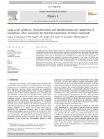
0.15 0.2 0.25 0.3 0.35 0.4
3

4
5
6
7
8
9
Tree stem diameter (m)
Traffic noise (cat.1, 70 km/h) IL (dBA)
FCC 2m
T 2m
SC 1m
SR 1m/2m
SR 2m/1m
SC 2m
SR 2m/3m
SR 3m/2m
SC 3m
Fig. 6. Average traffic noise IL (for a light vehicle at 70 km/h) in the receiver plane, in function of tree stem diameter, referenced to sound propagation
over grassland (receiver heights from 1 to 2 m). Different schemes were considered. The filling of the markers indicate whether the planting scheme is
realistic with ordinary tree plantings (white), if special measures needs to be taken (gray), or if the planting scheme will be hard to realize (black). See
Section 6 for discussion on this topic.
0 0.1 0.2 0.3 0.4 0.5 0.6 0.7 0.8 0.9 1
0
1
2
3
4
5
6
x (m)

Traffic noise IL (dBA)
30 km/h
40 km/h
50 km/h
60 km/h
70 km/h
80 km/h
90 km/h
100 km/h
110 km/h
120 km/h
Fig. 7. Traffic noise IL (dBA) along a representative part of planting scheme SR 1 m/2 m 22cm (at y¼2 m), for light vehicles at speeds ranging from 30 to
120 km/h. The reference situation is sound propagation over vegetation soil.
T. Van Renterghem et al. / Journal of Sound and Vibration 331 (2012) 2404–2425 2413
5.4. Effect of number of rows and stem height
In Fig. 8, the effect of the number of rows is considered for the SR 1 m/2 m scheme, for a tree stem diameter of 22 cm
and 44 cm. An increasing number of tree stems were removed, starting from the receiver plane. The vegetation soil was
replaced by grass-covered soil accordingly. In case of 2 rows, only close to the road trees are present. In case of 22-cm
diameter trees, a near-linear behavior is found when increasing the number of rows of trees, referenced to an identical soil
without trees. In case of a diameter of 44 cm, a large improvement is observed when going from 0 to 2 rows, which then
becomes linear when further increasing the number of rows.
With increasing tree height, the traffic noise shielding increases. However, the effect of stem height is rather
unimportant, once a height of 1 m is reached. Averaged over receiver heights from ground surface to 3 m, a difference
of about 1 dBA is observed for a stem height of 1 m high compared to 2.5 m, and for a stem diameter of 22 cm. Even low
stems perform well due to the presence of a source close to the vegetation area and close to the ground surface. Note that
tree crowns were absent when evaluating the importance of number of rows and stem height. The presence of
crowns below or at receiver height could be beneficial, compared to scattering from crowns above the receiver height
(see Section 1).
5.5. Effect of crown scattering
Since the exact distribution of biomass in a tree crown is not known, various approaches were tested as regards the

distribution of scattering elements to estimate the sensitivity of results on this choice. In the first 3 approaches, a 3rd order
power-law is used to relate the probability of filling a cell in function of the normalized distance towards the stem-axis.
The maximum probabilities at the stem axis are 0.5 (approach 1), 0.33 (approach 2) and 0.2 (approach 3). Next, a 5th order
(approach 4) and 7th order (approach 5) power law is applied, for a maximum probability of 0.5 at the stem axis.
The minimum probability at the sphere surface is 0.01 in all representations. Calculations are made for the lower half of
spherical tree crowns, starting at a height of 2.5 m, in absence of stems, above vegetation soil. Crowns organized as a SR
2 m setup are considered.
Scattering from tree crowns leads to an increase in sound pressure level and consequently a decrease in insertion loss.
The calculated insertion loss values, (linearly) averaged over the receiver plane at heights between 1 m and 2 m, are À0.8,
À0.5, À0.3, À0.6 and À0.4 dBA for approaches 1–5 (lower half of the tree crown only). It was numerically tested for
approach 1 that also including the upper half of the crown results in 0.2 dBA additional scattering.
0 1 2 3 4 5 6 7 8
0
1
2
3
4
5
6
7
Number of rows
Traffic noise (cat.1, 70 km/h)
IL (dBA)
y = 0−3m ref. veg./grass ground
y = 1−2m ref. veg./grass ground
y = 1−2m ref. grassland
0 1 2 3 4 5 6 7 8
0
2
4

6
8
10
Number of rows
Traffic noise (cat.1, 70 km/h)
IL (dBA)
0 0.5 1 1.5 2 2.5
0
1
2
3
4
5
6
7
Stem height (m)
Traffic noise (cat.1, 70 km/h)
IL (dBA)
0 0.5 1 1.5 2 2.5
0
2
4
6
8
10
Stem height (m)
Traffic noise (cat.1, 70 km/h)
IL (dBA)
Fig. 8. Total traffic noise IL for a light vehicle at 70 km/h, averaged over the receiver plane, in function of number of rows ((a) and (b)) and stem height
((c) and (d)). Results are referenced to sound propagation over vegetation soil (at heights between 0 and 3 m, and at heights between 1 and 2 m), and to

sound propagation over grassland (at heights between 1 and 2 m). The total length of the error bars equals two times the standard deviation. In (a) and
(c), planting scheme SR 1 m/2 m 22 cm is considered; in (b) and (d) planting scheme SR 1 m/2 m 44 cm.
T. Van Renterghem et al. / Journal of Sound and Vibration 331 (2012) 2404–24252414
Measurements of sound scattering by tree crowns behind a highway noise barrier (in a still atmosphere) [19] fall within
the range of the values predicted here. Simultaneous measurements were performed behind part of the noise barrier with
and without a (single) row of trees behind it. A log-linear relationship between sound frequency and level difference
between these two locations was measured (from þ0 dB at 1 kHz to þ5 dB at 10 kHz because of the crowns). When
applied to a light vehicle road traffic power spectrum at 70 km/h, this leads to an insertion loss value (of the tree crowns)
of À0.8 dBA. It can be concluded that the global effect of crown scattering is in qualitative agreement with measurements,
although scattering by leafs is not specifically addressed in the proposed numerical model.
5.6. Effect of shrubs
Two approaches were followed for comparing the effect of the presence of shrubs. First, the same amount of above-
ground biomass per unit area is modeled, distributed over shrubs with a height of 0.5 m, 1 m, 1.5 m and 2 m.
This corresponds to shrub porosities of 98 percent, 99 percent, 99.33 percent and 99.50 percent, respectively. Secondly,
two fixed shrub porosities were modeled, namely 99 percent and 99.5 percent. In the latter, the total amount of above-
ground biomass increases with shrub height.
For an equal amount of biomass, there is a preference for dense low vegetation as shown in Fig. 9. The minimum
performance that is observed for traffic noise shielding is for shrubs with a height near 1 m or 1.5 m, depending on
the receiver height zone considered. For a 2-m high shrub with the same amount of above-ground biomass, the traffic
noise shielding increases again. Note that the standard deviation when considering receiver heights from 0 to 3 m can be
quite high. More detailed analysis shows that for the more densely packed shrubs, positive effects for total traffic noise are
mainly observed for receivers above the shrub height. Zones with negative effects, mainly for the higher vehicle speeds,
were observed below the shrub height. For the 2-m high shrubs, such zones with negative effects do not appear.
For fixed shrub porosity, there is a preference for the 2-m high shrubs. For receiver heights between 1 m and 2 m, the
difference between 0.5 m, 1 m and 1.5 m shrubs is very similar, although there is 3 times as much vegetation mass for the
1.5-m shrubs compared to the 0.5-m shrubs.
A 2-m high shrub zone with a length of 15 m, for total above-ground dry biomass of 4 kg/m
2
, gives an average traffic
noise insertion loss of 4.7 dBA for a light vehicle at 70 km/h at typical ear heights (relative to sound propagation over

grassland). The positive effect of the presence of the ground is included here, accounting for 3.2 dBA. The effect of a soft
ground (developed by the presence of the shrubs) is therefore the major contribution to the traffic noise shielding.
Effects of different random realizations of the shrub layer are very minor (o 0.1 dBA) when considering averaged
results over the receiver planes for total traffic noise insertion loss.
5.7. Combining shrubs, crown scattering and the presence of stems
In this section, the acoustical effect of combinations of low (understorey) vegetation, crown scattering, and the
presence of stems are shown. Crown scattering approach 1 is applied. Shrubs of 0.5 m high with a porosity of 98 percent
0
1
2
3
4
5
6
7
8
9
10
H = 0.5m por = 98%
H = 1m por = 99%
H = 1.5m por = 99.33%
H = 2m por = 99.5%
H = 0.5m por = 99%
H = 1.5m por = 99%
H = 2m por = 99%
H = 0.5m por = 99.5%
H = 1m por = 99.5%
H = 1.5m por = 99.5%
Traffic noise (cat.1, 70 km/h) IL (dBA)
y = 0−3m ref. vegetation ground

y = 1−2m ref. vegetation ground
y = 1−2m ref. grassland
Fig. 9. Total traffic noise IL for a light vehicle at 70 km/h, averaged over the receiver plane, for shrubs above vegetation soil. Results are referenced to
sound propagation over vegetation soil (at heights between 0 and 3 m, and at heights between 1 and 2 m), and to sound propagation over grassland (at
heights between 1 and 2 m). The total length of the error bars equals two times the standard deviation.
T. Van Renterghem et al. / Journal of Sound and Vibration 331 (2012) 2404–2425 2415
are used. SC 2 m tree planting schemes are applied, with diameters of 22 cm and 44 cm. Identical realizations are used for
the crowns and low vegetation in the different combinations.
In Fig. 10, explicitly modeled combinations are shown and compared to the result of adding the insertion losses of
single effects (i.e. stems only with a diameter of 22 cm or 44 cm, shrubs only, and tree crowns only). Effects of stems,
crown scattering and low vegetation can be considered as more or less additive based on these simulations, when
considering sound propagation referenced to the same type of soil. Adding insertion losses of separate effects, and
comparing the results to explicitly modeling combinations, yield differences of at most 0.7 dBA (averaged over receiver
heights from 1 to 2 m). It is clear that additivity does not hold when referenced to sound propagation over grassland, since
the positive ground effect is included in all parts. These findings show that the different parts in vegetation belts only
interact to a limited extent when considering typical road traffic noise spectra. As a result, it does not seem necessary to
perform simulations of combinations of understorey vegetation, different stem schemes and crown representations to
have an adequate estimate of the global effect.
This additivity of scattering by vegetation and the sound–soil interaction is consistent with the findings in Refs. [1,31],
and could potentially lead to simplified and less computationally intensive approaches than the one used in this study.
Note that the shrub mass density per unit area assumed here exceeds what would be practically possible as an
understorey in a (dense) tree stand. However, the main purpose of this section was checking possible interactions between
the different layers in a vegetation belt.
5.8. Randomization and lattice defects
The presence of (some) randomness in the stem center location and stem diameter will be inherent in practical
realizations of tree belts. Secondly, sonic crystal research showed that positive effects could be expected by inducing
lattice defects in case of densely packed cylinders, leading to a broadening of insertion loss peaks [34]. Since road traffic
noise spectra are characterized by a broad frequency range, this effect is worth studying.
The use of the reflecting plane approach as applied in this numerical study can only lead to periodic planting schemes
along the road axis. Only the effect of random shifts orthogonal to the road can be studied.

5.8.1. Shifts in stem center location
In a first step, the effect of random shifts in stem center location is studied for some schemes with a spacing of 2 m
normal to the road. It is clear that complete randomness is not of practical use, since it conflicts with the minimum
planting distance needed for development of neighboring trees. Random shifts up to 0.75 m were allowed normal to the
road and in both directions, compared to a constant spacing. Three random realizations are considered in each case and the
insertion losses were linearly averaged afterwards.
−1
0
1
2
3
4
5
6
7
shrubs + crowns
stems 22cm + shrubs
stems 44cm + shrubs
stems 22cm + crowns
stems 44cm + crowns
stems 22cm + shrubs + crowns
stems 44cm + shrubs + crowns
Traffic noise (cat.1, 70 km/h)
IL (dBA)
explicitly simulated
assuming additivity
Fig. 10. Total traffic noise IL for a light vehicle at 70 km/h, averaged over the receiver plane, for combinations of shrubs (H¼0.5 m, por¼0.98), stems (SC
2 m 22 cm and SC 2 m 44 cm), and tree crowns (approach 1) above vegetation soil. Explicitly simulated combinations are compared to the result of
adding the insertion losses of single effects. Results are referenced to sound propagation over vegetation soil (at heights between 1 and 2 m). The total
length of the error bars equals two times the standard deviation.

T. Van Renterghem et al. / Journal of Sound and Vibration 331 (2012) 2404–24252416
Inducing some (pseudo)randomness in the location of the stem center is predicted not to decrease traffic noise
insertion loss as illustrated in Fig. 11. In the more densely packed SR 1 m/2 m 44 cm scheme, an increase in traffic noise
insertion loss near 0.5 dBA is observed. For the SC 2 m scheme, the additional positive effect of randomness in stem center
location is very limited.
5.8.2. Randomness in tree diameter
In a SR 1 m/2 m scheme, random variations in tree stem diameter are modeled, ranging from 22 cm to 44 cm, following
a uniform distribution. The (linearly) averaged traffic noise insertion loss of 3 such realizations (referenced to vegetation
soil, for receivers between 0 and 3 m) shows a noise reducing potential (3.9 dBA) that is closer to the performance of a
uniform 44-cm diameter tree stand (5.0 dBA) than to the uniform 22-cm diameter tree stand (2.3 dBA). Similarly, for SC
2 m, mixing diameters lead to a traffic noise insertion loss of 2.1 dBA, which is again closer to the uniform 44-cm diameter
tree stand (2.5 dBA) than to the uniform 22-cm diameter stand (1.4 dBA). This shows that randomness in tree diameter is
positive from the viewpoint of noise reduction. Selecting for identical trees should therefore not be encouraged.
5.8.3. Including gaps
The effect of omitting some rows for planting schemes SR 1 m/2 m is simulated, with fixed stem diameters of either
22 cm or 44 cm. Four different realizations of 2 missing rows were simulated and compared to using 8 rows to fill the zone
designed for the planting scheme (see Fig. 12). Leaving out some rows does not significantly influence the averaged traffic
noise insertion loss in the receiver plane. Some of such realizations including gaps seem to even improve noise shielding a
0
1
2
3
4
5
6
7
8
9
10
SR 1m/2m 44cm

SR 1m/2m 44cm R
SR 1m/2m 22cm
SR 1m/2m 22cm R
SC 2m 44cm
SC 2m 44cm R
SC 2m 22cm
SC 2m 22cm R
Traffic noise (cat.1, 70 km/h) IL (dBA)
y = 0−3m ref. vegetation ground
y = 1−2m ref. vegetation ground
y = 1−2m ref. grassland
Fig. 11. Total traffic noise IL for a light vehicle at 70 km/h, averaged over the receiver plane, for different schemes, including random shifts in stem center
location (indicated by ‘‘R’’). Results are referenced to sound propagation over vegetation soil (at heights between 0 and 3 m, and at heights between 1 and
2 m), and to sound propagation over grassland (at heights between 1 and 2 m). The total length of the error bars equals two times the standard deviation.
Fig. 12. The 4 realizations considered (shown as representative strips) in case of 2 missing rows out of 8 (a)–(d). The fully populated grid is shown in (e).
S and R indicate the source and receiver side, respectively.
T. Van Renterghem et al. / Journal of Sound and Vibration 331 (2012) 2404–2425 2417
little (realizations a and d: þ0.2 dBA) for the tree diameter of 44 cm (referenced to sound propagation over grassland, and
receiver heights between 1 m and 2 m). For the 22-cm diameter stems, there is a small reduction (at maximum À0.3 dBA)
in insertion loss. Similar conclusions could be drawn by considering SC 2 m. Omitting some rows in between the tree stand
is better for noise shielding than, e.g. limiting two rows at the end, as shown in Fig. 8. It is assumed that near these open
spaces, a vegetation soil is developed as well, which is not expected in case of limiting the tree belt to 6 consecutive rows.
It is discussed in Section 6 that this finding is interesting for the practical realization of tree stands.
5.9. Sound propagation over rigid thin noise barrier
For comparison, the FDTD model applying mirror planes is used to calculate the insertion loss of a rigid rectangular
screen with a thickness of 0.1 m, placed at 3 m relative to the source position. In this approach, the screen is infinitely long
and parallel to the road axis. The screen is placed on grass-covered ground, and road traffic noise levels are referenced to
sound propagation over unscreened grassland. The noise shielding by vegetation belts is referenced to grassland as well.
Screen heights of 0.5 m, 1.0 m, 1.5 m, 2.0 m, and 2.5 m were considered. The insertion losses obtained (for receivers
between 1 m and 2 m, and a vehicle speed of 70 km/h) are 3.6, 6.2, 8.8, 10.6, and 11.7 dBA, respectively. Some of the

vegetation schemes that can be practically realized (see Section 6) could compete with a screen of 1 m or even 1.5 m.
An important reason is the preservation and change of the ground effect when vegetation is used. In case of a classical
screen, this positive ground effect can be (partly) lost by preventing the direct and ground-reflected wave to destructively
interfere. Note that the screen calculations are performed for a coherent line source. Noise barrier shielding in case of an
incoherent line source is expected to be lower [57,58] than the results shown here. This fortifies the conclusions drawn.
Furthermore, classical noise barriers are sensitive to an important decrease in shielding in case of downwind sound
propagation, even at short distance [59,60]. In case of a stand of vegetation, such negative effects are expected to a much
lesser extent since vegetation acts as a windbreak; the strong vertical gradients in the horizontal component of the wind
speed as observed near the barrier top [21] will not appear.
6. Practical considerations
Well-established empirical relationships exist between the number of trees per unit area and their stem diameter [61].
Based on such relationships, the suggested tree density–tree diameter combinations considered in this work are not all
realistic in ordinary tree plantings, especially for the stems with a diameter of 44 cm. Such results are nevertheless kept in
the analysis to reveal trends. Following findings in this study are interesting from the practical point of view.
Firstly, numerical simulations indicated that omitting some rows of trees does not affect the traffic noise insertion loss
of the tree stand. Trees planted in densely clustered zones followed by open spaces could therefore be practically
achievable, as this ensures that more resources (light, water and nutrients) are available for tree growth and that higher
tree densities can be obtained.
Secondly, there is a preference for rectangular schemes, for stem diameters of 22 cm. The noise reduction obtained by
scheme SR 2 m/3 m is close to the one of SC 2 m, although SR 2 m/3 m has a smaller tree density (0.17 m
À2
) than SC 2 m
(0.25 m
À2
). It was further shown that the orientation in rectangular schemes, relative to the road axis, is important:
SR 3 m/2 m and SR 2 m/3 m have the same tree density, however, SR 2 m/3 m is preferred. The SR 3 m/2 m scheme has
only the acoustic performance of SC 3 m.
Thirdly, pollarded trees are of special interest as they can attain large stem diameters at high densities and they have a
limited amount of biomass in the canopy due to the cyclic removal of the branches and foliage. As a result, the possible
negative effects of downward scattering will be limited. Another interesting property is that many tree genera suitable for

pollarding (e.g. Salix and Populus) are fast growing. In case high stem diameters can be realized and one has to deal with
high-speed road traffic, a FCC scheme should be preferred upon a SC scheme: for a same tree density, a higher insertion
loss is obtained.
It is indicated in Fig. 6 whether the combinations of planting schemes, tree spacing, and tree stem diameters are
practically achievable. Given the complexity in assessing this, three categories were defined based on the considerations in
previous sections. When the surface taken by the stem cross-sections is smaller than 100 m
2
/ha (equivalent to 1 percent
stem cover), no practical problems are expected (white-filled markers). At the other hand, values above 2 percent are
considered to be rather unrealistic (black-filled markers). Between 1 percent and 2 percent, tree belts might be achieved
when selecting for species that can be densely planted or develop large stem diameters. Another option is leaving out
some rows to obtain an averaged smaller tree base area density (note that the values given here are based on fully
populated grids).
The highest total A-weighted road traffic noise insertion loss (on condition that the stem cross-section area stays below
1 percent) is observed when applying a SC 1 m 11 cm scheme. Another practical solution is a SR 2 m/3 m 22 cm scheme: a
performance equivalent to a noise barrier with a height of 1 m on grassland is possible, when also allowing for a shrub
layer. For a light vehicle at 70 km/h, a traffic noise reduction of near 5 dBA can be achieved (without a shrub layer) with
a limited belt depth of only 15 m. Such a scheme can be realized with common species, and has a basal area of only
63 m
2
/ha. The FCC 2 m 22 cm has a traffic noise insertion loss which is 0.5 dBA higher, however, the stem base areal
T. Van Renterghem et al. / Journal of Sound and Vibration 331 (2012) 2404–24252418
density is very close (95 m
2
/ha) to the maximum set value here. Tree stems with diameters of 44 cm are less interesting
when combining acoustical efficiency and practical achievability.
7. Conclusions
In this study, the 3D finite-difference time-domain method is used to simulate sound propagation through an infinitely
long and 15-m deep vegetation belt along a road. A representative strip of the vegetation belt is considered and mirror
planes are placed at the simulation boundaries, normal to the road axis. Preliminary calculations showed that the latter is a

sound approach to model an infinitely wide vegetation belt. The computational cost was further reduced by showing that
for this specific application and when averaging over a receiver zone, assigning the engine and rolling noise source power
to the engine noise source height only (in the Harmonoise/Imagine road traffic noise emission model) was sufficiently
accurate. Furthermore, calculations have been performed for coherent line sources. The use of a (partly) incoherent line
source generally results in a slightly increased road traffic insertion loss by the vegetation belt.
The presence of a forest floor alone, compared to sound propagation over grassland, was found to be responsible for a
reduction in total traffic noise level for a light vehicle driving at 70 km/h near 3 dBA. The noise reducing effects of the
forest floor and the optimal tree stem configuration (among the modeled ones), taking into account practical achievability,
were predicted to be of similar importance.
With increasing tree stem diameter, traffic noise insertion loss is more pronounced for each planting scheme
considered. Furthermore, with increasing distance between the stems, smaller values were found and the importance of
the stem diameter decreases. A tree spacing of 3 m and a stem diameter of 11 cm can be considered as the starting point of
having positive effects (near 0.5 dBA for a light vehicle at 70 km/h). Note that even for such sparse vegetation, positive
ground effects could be expected. The spacing parallel to the road axis was shown to be most important in predicting road
traffic noise shielding.
To model the interaction between sound and shrubs, a uniform distribution of scattering cells is assumed. The porosity
taken by woody shrub material is estimated based on typical values for the above-ground biomass per unit surface area
and allometric relationships. A 2 m-high shrub zone with a length of 15 m, for total above-ground dry biomass of 4 kg/m
2
,
gives an average road traffic noise insertion loss of 4.7 dBA for a light vehicle at 70 km/h at typical ear heights
when referenced to sound propagation over grassland. For an equal amount of biomass per unit surface area, there is
a preference for either low shrubs (0.5 m) or higher shrubs (2 m).
Scattering from tree crowns leads to downward scattering of sound, given the low source height and receiver height
below the canopy, at close distance. Depending on the parameters used for the specific distribution of scattering elements
in the tree crown, the predicted negative effects range from À0.8 to À0.4 dBA for a light vehicle at 70 km/h. With
increasing vehicle speed, downward scattering increases. Measurements of road traffic noise scattering near a highway
noise barrier including a row of trees (described in another study) fall in the predicted range.
The effect of the presence of tree crowns, shrubs and tree stems was found to be approximately additive. Errors made
by adding the insertion losses of the individual layers in the vegetation belt, and thus not explicitly modeling

combinations, were smaller than 0.7 dBA for receiver heights ranging from 1 m to 2 m.
Simulations showed that inducing some (pseudo)randomness, either in stem center location, tree diameter, or by
omitting a number of rows (assuming that the same forest floor develops in the open zones) hardly affects the insertion
loss values. This is interesting from the viewpoint of practical realizations of tree stands, given the inherent randomness in
working with living material. Note that in the current mirror-plane approach, only randomness in a direction normal to
the road could be considered. Furthermore, omitting some rows in a tree stem grid could allow for local denser zones, still
having realistic averaged stem base areal densities. It could be concluded that realistically achievable 15-m deep
vegetation belts could compete with the traffic noise insertion loss of a thin, classical noise barrier (on grassland) with a
height of 1–1.5 m in a non-refracting atmosphere. The vegetation belt has additional non-acoustic advantages such as
being CO
2
-neutral or positive, having a much higher esthetic value, and its potential to improve local air quality, e.g. by
capturing road traffic-originated fine particles.
As a final remark, it has to be stressed that the current study is a purely numerical one. Although a full-wave 3D
numerical model has been used, and input parameters in the model are as much as possible based on measured data,
validation with measurements at vegetation belts is not provided.
Acknowledgment
The research leading to these results has received funding from the European Community’s Seventh Framework
Program (FP7/2007–2013) under grant agreement no. 234306, collaborative project HOSANNA.
Appendix A. Testing mirror plane approach
The mirror plane approach is checked by means of two dimensional calculations. Insertion loss values for 1/3-octave
bands (with central frequencies ranging from 25 Hz to 1600 Hz) using a representative strip only in between two perfectly
T. Van Renterghem et al. / Journal of Sound and Vibration 331 (2012) 2404–2425 2419
reflecting planes are compared to the results of explicitly modeling a wide strip applying the same scheme. This wide strip
is also bordered by reflecting planes at the simulation boundaries along the x-axis. In such 2D calculations, coherent plane
waves are modeled, parallel to the infinitely long cylinders, in absence of a reflecting ground plane. The number of time
steps is kept the same in both situations to have the same amount of reflected energy.
In Fig. A.1, the insertion loss spectrum is shown in the middle of the minimal representative strip of an SR 1 m/2 m
44 cm scheme consisting of partly absorbing cylinders (bark impedance). The corresponding data in case of an explicitly
modeled wider strip is shown as well. The results are in good agreement. Only at higher frequencies, small differences are

observed. Receiver patterns of insertion losses are also repeated when a wide strip is modeled (not shown).
Appendix B. Calculations with two source heights vs. single source height
The Harmonoise/Imagine (H/I) source power model needs calculations for two source heights. However, since this
doubles the number of calculations needed to assess traffic noise insertion loss, it is checked whether the total traffic noise
source power (which is the energetic frequency-dependent sum of rolling noise and engine noise) could be assigned
completely to the highest source position. For comparison, the H/I model is applied as prescribed, namely sound
propagation from both the rolling noise height and engine noise height is explicitly modeled, and the dedicated source
power level is assigned to the corresponding source heights, and finally results are energetically summed.
Fig. B.1 shows the average IL in the receiver plane for a type 1 vehicle (light vehicles) as a function of driving speed,
calculated with one and two source heights, respectively. When referenced to grassland, taking into account calculations
at two source heights, results in slightly higher insertion losses (o 0.5 dBA), especially at the higher vehicle speeds.
The single source height approach is therefore considered as sufficiently accurate and is applied in this numerical study,
and will result in a slight underprediction of traffic noise insertion losses. Averaging over a range of receiver heights is
a possible reason that relaxes the need to explicitly model multiple source heights.
Appendix C. Effect of source type
An incoherent line source is a better representation of a traffic line source. Therefore, the effect of introducing
incoherence in the source is compared to a fully coherent line source for some planting schemes. This is modeled in FDTD
by assigning a random phase at each point source constituting the line source. In case of a coherent line source, on the
other hand, all these pressure points are in phase. In the representative strip approach, however, only incoherence in
the representative strip can be modeled. Giving the fact that both the source and planting scheme are mirrored by the
reflecting planes at x¼0 and w
rs
, a partly incoherent line source is actually modeled. The mirrored part of the line source is
again in phase with the explicitly modeled part of the line source. However, this approach allows studying the importance
of source type.
Given the random nature involved, each simulation for the partly incoherent line source is performed for 5 realizations
and (linearly) averaged afterwards. The influence of source type has been investigated for 3 different planting schemes,
each time for a stem diameter of 22 cm and 44 cm. The difference in average insertion loss between a coherent and (partly)
incoherent line source, in function of vehicle speed, is shown in Fig. C.1.
10

2
10
3
0
2
4
6
8
10
12
14
16
Frequency (Hz)
IL (dB)
explicitly modelled wide strip
mirror plane approach
Fig. A.1. Coherent plane wave insertion loss spectrum of a representative strip (using the mirror plane approach) and an explicitly modeled wide SC 1 m/
2 m 44 cm grid. Absorbing cylinders were considered.
T. Van Renterghem et al. / Journal of Sound and Vibration 331 (2012) 2404–24252420
It can be concluded that an incoherent line source does not result in overall lower insertion loss values when compared
to the same type of ground, in contrast to what is observed, e.g. near noise screens [57,58]. In most cases, the incoherent
line source representation gives a somewhat higher traffic noise insertion loss. Furthermore, this difference is vehicle-
speed dependent. Only for the SR 1 m/2 m 22 cm scheme, a coherent line source gives a slightly higher insertion loss at
vehicle speeds exceeding 70 km/h. The averaged differences are mostly limited to within 1 dBA. Modeling a coherent line
source as is performed in this paper will typically lead to a slight underprediction of the traffic noise insertion loss.
30 40 50 60 70 80 90 100 110 120
5
6
7
8

9
10
11
12
Vehicle speed (km/h)
Traffic noise IL (dBA)
one source height
two source heights
Fig. B.1. Difference in averaged traffic noise IL (referenced to grass-covered soil) for a simulation using a single source height and two source heights as
prescribed by the H/I road traffic source power model. The SR 1 m/2 m 44 cm scheme is considered, with receiver heights between 1 m and 2 m. The
dashed lines show the minimum and maximum IL found in the receiver plane. The error bars have a total length of two times the standard deviation.
30 40 50 60 70 80 90 100 110 120
−2
−1
0
1
2
3
IL
coh
−IL
incoh
(dBA)
30 40 50 60 70 80 90 100 110 120
−2
−1
0
1
2
3

30 40 50 60 70 80 90 100 110 120
−2
−1
0
1
2
3
IL
coh
−IL
incoh
(dBA)
30 40 50 60 70 80 90 100 110 120
−2
−1
0
1
2
3
30 40 50 60 70 80 90 100 110 120
−2
−1
0
1
2
3
vehicle speed (km/h)
IL
coh
−IL

incoh
(dBA)
30 40 50 60 70 80 90 100 110 120
−2
−1
0
1
2
3
vehicle speed (km/h)
Fig. C.1. Difference in traffic noise IL (light vehicle) between a coherent line source and a (partly) incoherent line source, averaged over the receiver plane
(for receivers between 1 m and 2 m), with increasing vehicle speed. The error bars have a total length of two times the standard deviation. The reference
situation is here sound propagation over ground as appears under vegetation. Schemes considered: (a) T 2 m 44 cm, (b) T 2 m 22 cm, (c) SR 1 m/2 m
44 cm, (d) SR 1 m/2 m 22 cm, (e) SC 2 m 44 cm and (f) SC 2 m 22 cm.
T. Van Renterghem et al. / Journal of Sound and Vibration 331 (2012) 2404–2425 2421
Table D1
Overview of simulation results for total traffic noise reduction (in dBA) of different tree stems orderings and parameters, for light vehicle speeds of 30 km/h, 70 km/h, and 110 km/h, referenced to sound
propagation over the same type of soil (vegetation soil) or grassland, in absence of tree stems. The values in between brackets are the standard deviation on the data in the receiver zones considered. A coherent
line source is used. Stem diameters are constant, and shifts of the stem axis from the planting scheme considered are absent unless explicitly indicated. Details on the exact locations of the gaps are found in
Fig. 12; the parameter choice as for the randomness in stem center location and diameter can be found in Section 5.8.
Scheme Spacing Stem
diameter (cm)
Stem height
(m)
Number of
rows
Additional
information
30 km/h 70 km/h 110 km/h
Veg. soil

(0–3 m)
Veg. soil
(1–2 m)
Grass
(1–2 m)
Veg. soil
(0–3 m)
Veg. soil
(1–2 m)
Grass
(1–2 m)
Veg. soil
(0–3 m)
Veg. soil
(1–2 m)
Grass
(1–2 m)
FCC 2 m 11 2.5 11 0.2 (0.1) 0.3 (0.1) 3 (0.1) 0.8 (0.3) 1 (0.2) 4.2 (0.4) 1.1 (0.4) 1.4 (0.3) 4.7 (0.7)
FCC 2 m 22 2.5 11 0.5 (0.2) 0.5 (0.1) 3.3 (0.1) 1.5 (0.6) 1.9 (0.3) 5.1 (0.4) 2.2 (0.8) 2.8 (0.5) 6.1 (0.7)
FCC 2 m 44 2.5 11 0.8 (0.6) 0.9 (0.2) 3.6 (0.1) 2.5 (1.1) 2.9 (0.4) 6.1 (0.2) 3.8 (1.3) 4.5 (0.4) 7.8 (0.5)
SC 1 m 11 2.5 16 0.6 (0.1) 0.7 (0.1) 3.4 (0.1) 1.6 (0.6) 2.1 (0.2) 5.3 (0.4) 2.4 (0.8) 3.1 (0.3) 6.4 (0.7)
SC 1 m 22 2.5 16 1.1 (0.5) 1.1 (0.2) 3.8 (0.1) 2.6 (1.1) 2.8 (0.3) 6.1 (0.4) 3.7 (1.3) 4.2 (0.5) 7.5 (0.8)
SC 1 m 44 2.5 16 2.5 (1.8) 2.4 (0.7) 5.1 (0.5) 4.7 (2.7) 4.8 (0.8) 8 (0.4) 6.6 (3) 6.9 (0.7) 10.2 (0.3)
SC 2 m 11 2.5 8 0.2 (0.1) 0.3 (0.1) 3 (0.1) 0.7 (0.5) 0.9 (0.5) 4.1 (0.6) 1 (0.7) 1.3 (0.7) 4.6 (0.9)
SC 2 m 22 2.5 6 Gaps, realization a 0.5 (0.2) 0.5 (0.1) 3.3 (0.1) 1.3 (0.5) 1.6 (0.3) 4.8 (0.4) 1.8 (0.6) 2.2 (0.4) 5.5 (0.7)
SC 2 m 22 2.5 6 Gaps, realization b 0.5 (0.2) 0.5 (0.1) 3.2 (0.1) 1.2 (0.6) 1.5 (0.4) 4.8 (0.5) 1.7 (0.8) 2.1 (0.6) 5.5 (0.9)
SC 2 m 22 2.5 6 Gaps, realization c 0.5 (0.2) 0.5 (0.1) 3.2 (0.1) 1.2 (0.5) 1.5 (0.3) 4.7 (0.5) 1.6 (0.6) 2 (0.4) 5.3 (0.7)
SC 2 m 22 2.5 6 Gaps, realization d 0.5 (0.2) 0.5 (0.1) 3.3 (0.1) 1.3 (0.6) 1.6 (0.4) 4.8 (0.5) 1.8 (0.8) 2.2 (0.7) 5.5 (0.9)
SC 2 m 22 2.5 8 Stem center shifts 0.6 (0.3) 0.6 (0.1) 3.3 (0.1) 1.5 (0.6) 1.9 (0.4) 5.1 (0.4) 2.1 (0.8) 2.6 (0.5) 5.9 (0.8)
SC 2 m 22 2.5 8 0.6 (0.2) 0.6 (0.1) 3.3 (0.1) 1.4 (0.6) 1.8 (0.3) 5 (0.4) 2 (0.7) 2.5 (0.5) 5.8 (0.7)

SC 2 m 44 2.5 6 Gaps, realization a 1.3 (0.3) 1.4 (0.1) 4.1 (0.1) 2.4 (0.8) 2.7 (0.4) 6 (0.5) 3.2 (0.9) 3.6 (0.7) 6.9 (0.9)
SC 2 m 44 2.5 6 Gaps, realization b 1.3 (0.3) 1.4 (0.1) 4.1 (0.1) 2.5 (0.8) 2.8 (0.4) 6 (0.5) 3.3 (0.9) 3.7 (0.7) 7 (0.9)
SC 2 m 44 2.5 6 Gaps, realization c 1.4 (0.4) 1.4 (0.2) 4.1 (0.1) 2.5 (0.9) 2.8 (0.6) 6 (0.7) 3.3 (1.1) 3.7 (1) 7 (1.2)
SC 2 m 44 2.5 6 Gaps, realization d 1.4 (0.3) 1.4 (0.1) 4.1 (0.1) 2.5 (0.8) 2.8 (0.5) 6 (0.5) 3.3 (1) 3.7 (0.8) 7 (0.9)
SC 2 m 44 2.5 8 Stem center shifts 1.4 (0.4) 1.5 (0.2) 4.2 (0.1) 2.6 (0.9) 2.9 (0.6) 6.2 (0.6) 3.5 (1.2) 3.9 (1) 7.2 (1.2)
SC 2 m 44 2.5 8 1.5 (0.4) 1.5 (0.2) 4.3 (0.1) 2.5 (1) 2.7 (0.7) 6 (0.8) 3.2 (1.3) 3.5 (1.2) 6.9 (1.3)
SC 2 m 22–44 2.5 8 Random stem diameter 1 (0.3) 1 (0.1) 3.8 (0.1) 2.1 (0.8) 2.4 (0.5) 5.6 (0.5) 2.8 (1) 3.2 (0.8) 6.6 (1)
SC 3 m 22 2.5 6 0.3 (0.1) 0.3 (0.1) 3 (0.1) 0.7 (0.4) 0.9 (0.4) 4.1 (0.6) 1 (0.6) 1.2 (0.7) 4.6 (0.9)
SC 3 m 44 2.5 6 0.8 (0.2) 0.8 (0.1) 3.5 (0.1) 1.5 (0.9) 1.6 (1) 4.9 (1) 2 (1.4) 2.3 (1.6) 5.6 (1.7)
SC 3 m 11 2.5 6 0.1 (0.1) 0.1 (0.1) 2.9 (0.1) 0.3 (0.2) 0.4 (0.2) 3.7 (0.5) 0.5 (0.3) 0.6 (0.2) 3.9 (0.7)
SR 1 m/2 m 11 2.5 8 0.4 (0.1) 0.5 (0.1) 3.2 (0.1) 1.1 (0.4) 1.4 (0.2) 4.7 (0.4) 1.6 (0.5) 2 (0.3) 5.3 (0.6)
SR 1 m/2 m 22 2.5 2 0.5 (0) 0.5 (0) 1.5 (0) 1.1 (0.2) 1.1 (0.1) 3.1 (0.1) 1.4 (0.2) 1.5 (0.2) 3.9 (0.2)
SR 1 m/2 m 22 2.5 4 0.7 (0.1) 0.6 (0.1) 2.2 (0.1) 1.7 (0.4) 1.7 (0.2) 4.4 (0.2) 2.4 (0.5) 2.5 (0.3) 5.6 (0.4)
SR 1 m/2 m 22 2.5 6 Gaps, realization a 0.9 (0.2) 1 (0.1) 3.7 (0.1) 2.2 (0.8) 2.7 (0.3) 5.9 (0.3) 3.2 (1) 3.9 (0.4) 7.2 (0.6)
SR 1 m/2 m 22 2.5 6 Gaps, realization b 0.8 (0.2) 0.9 (0.1) 3.6 (0.1) 2.1 (0.7) 2.5 (0.3) 5.8 (0.4) 3 (0.9) 3.7 (0.5) 7 (0.7)
SR 1 m/2 m 22 2.5 6 Gaps, realization c 0.8 (0.2) 0.9 (0.1) 3.6 (0.1) 2 (0.7) 2.4 (0.3) 5.7 (0.4) 2.8 (0.9) 3.4 (0.5) 6.8 (0.8)
SR 1 m/2 m 22 2.5 6 Gaps, realization d 0.9 (0.2) 0.9 (0.1) 3.7 (0.1) 2.1 (0.7) 2.6 (0.3) 5.8 (0.4) 3 (0.9) 3.7 (0.4) 7 (0.7)
SR 1 m/2 m 22 2.5 6 0.8 (0.2) 0.8 (0.1) 2.7 (0.1) 2 (0.6) 2.2 (0.3) 5.1 (0.2) 2.8 (0.7) 3.3 (0.4) 6.4 (0.4)
SR 1 m/2 m 22 0.5 8 0.3 (0.2) 0.4 (0.1) 3.1 (0.1) 0.9 (0.3) 1.1 (0.1) 4.4 (0.4) 1.2 (0.4) 1.6 (0.1) 4.9 (0.6)
SR 1 m/2 m 22 1 8 0.6 (0.4) 0.7 (0.1) 3.4 (0) 1.5 (0.8) 2 (0.3) 5.2 (0.3) 2.1 (1) 2.8 (0.3) 6.2 (0.6)
SR 1 m/2 m 22 1.5 8 0.7 (0.4) 0.8 (0.2) 3.5 (0.1) 1.8 (1) 2.2 (0.5) 5.4 (0.2) 2.5 (1.2) 3.2 (0.6) 6.5 (0.4)
SR 1 m/2 m 22 2 8 0.8 (0.4) 0.8 (0.2) 3.6 (0.1) 2 (0.9) 2.3 (0.4) 5.5 (0.4) 2.9 (1.1) 3.3 (0.5) 6.6 (0.7)
SR 1 m/2 m 22 2.5 8 Stem center shifts 1 (0.3) 1 (0.1) 3.8 (0) 2.6 (0.9) 3.1 (0.3) 6.3 (0.3) 3.8 (1.2) 4.6 (0.4) 8 (0.6)
SR 1 m/2 m 22 2.5 8 1 (0.3) 1 (0.1) 3.8 (0.1) 2.3 (0.8) 2.8 (0.3) 6 (0.4) 3.2 (1) 4 (0.5) 7.3 (0.7)
SR 1 m/2 m 44 2.5 2 1.9 (0.1) 1.9 (0.1) 2.9 (0.1) 2.9 (0.3) 3 (0.3) 5 (0.3) 3.6 (0.5) 3.7 (0.5) 6.1 (0.5)
SR 1 m/2 m 44 2.5 4 2.5 (0.2) 2.5 (0.1) 4 (0.1) 3.8 (0.6) 3.9 (0.3) 6.5 (0.2) 4.8 (0.7) 5 (0.5) 8 (0.4)
SR 1 m/2 m 44 2.5 6 Gaps, realization a 3.2 (0.4) 3.2 (0.2) 5.9 (0.1) 4.9 (1.1) 5.3 (0.4) 8.6 (0.2) 6.3 (1.3) 7 (0.4) 10.4 (0.6)
T. Van Renterghem et al. / Journal of Sound and Vibration 331 (2012) 2404–24252422
SR 1 m/2 m 44 2.5 6 Gaps, realization b 3.1 (0.5) 3.2 (0.2) 5.9 (0.1) 4.8 (1.1) 5.2 (0.4) 8.4 (0.3) 6.2 (1.3) 6.7 (0.4) 10.1 (0.6)
SR 1 m/2 m 44 2.5 6 Gaps, realization c 3.3 (0.5) 3.3 (0.2) 6 (0.1) 4.7 (1.1) 5 (0.4) 8.2 (0.3) 5.8 (1.2) 6.2 (0.5) 9.6 (0.7)

SR 1 m/2 m 44 2.5 6 Gaps, realization d 3.3 (0.4) 3.3 (0.2) 6 (0.1) 5 (1.1) 5.3 (0.4) 8.6 (0.3) 6.4 (1.3) 7 (0.4) 10.3 (0.6)
SR 1 m/2 m 44 2.5 6 2.9 (0.5) 2.9 (0.2) 4.9 (0.2) 4.3 (1) 4.5 (0.5) 7.4 (0.2) 5.3 (1.3) 5.9 (0.6) 9 (0.4)
SR 1 m/2 m 44 0.5 8 1.1 (0.3) 1.2 (0.1) 3.9 (0) 2 (0.6) 2.5 (0.1) 5.7 (0.4) 2.8 (0.7) 3.4 (0.1) 6.8 (0.7)
SR 1 m/2 m 44 1 8 2.2 (0.7) 2.4 (0.3) 5.1 (0.2) 3.8 (1.3) 4.6 (0.4) 7.8 (0.2) 5 (1.6) 6.4 (0.3) 9.7 (0.5)
SR 1 m/2 m 44 1.5 8 2.8 (0.9) 3 (0.4) 5.7 (0.3) 4.5 (1.7) 5.3 (0.7) 8.5 (0.3) 5.8 (2.1) 7.1 (0.9) 10.4 (0.5)
SR 1 m/2 m 44 2 8 3.2 (0.9) 3.2 (0.4) 5.9 (0.3) 4.8 (1.7) 5.1 (0.7) 8.3 (0.4) 6 (2) 6.5 (0.9) 9.8 (0.5)
SR 1 m/2 m 44 2.5 8 Stem center shifts 3.3 (0.7) 3.3 (0.3) 6.1 (0.2) 5.4 (1.5) 5.7 (0.5) 8.9 (0.1) 7.1 (1.7) 7.8 (0.4) 11.1 (0.3)
SR 1 m/2 m 44 2.5 8 3.5 (0.7) 3.5 (0.3) 6.2 (0.2) 5 (1.4) 5.2 (0.5) 8.4 (0.3) 6.1 (1.6) 6.5 (0.6) 9.8 (0.6)
SR 1 m/2 m 22–44 2.5 8 Random stem diameter 2.1 (0.5) 2.2 (0.2) 4.9 (0.1) 3.9 (1.2) 4.2 (0.4) 7.5 (0.2) 5.1 (1.4) 5.8 (0.4) 9.2 (0.5)
SR 1 m/3 m 11 2.5 6 0.3 (0.1) 0.4 (0.1) 3.1 (0.1) 0.9 (0.4) 1.2 (0.2) 4.4 (0.4) 1.3 (0.5) 1.7 (0.3) 5 (0.7)
SR 1 m/3 m 22 2.5 6 0.8 (0.2) 0.9 (0.1) 3.6 (0.1) 2.1 (0.7) 2.5 (0.3) 5.8 (0.4) 3 (0.9) 3.8 (0.4) 7.1 (0.7)
SR 1 m/3 m 44 2.5 6 2.6 (0.4) 2.6 (0.2) 5.3 (0.1) 4.3 (1) 4.7 (0.4) 8 (0.5) 5.9 (1.3) 6.6 (0.6) 9.9 (0.8)
SR 2 m/1 m 11 2.5 8 0.4 (0.1) 0.5 (0.1) 3.2 (0.1) 1.1 (0.5) 1.5 (0.3) 4.7 (0.5) 1.6 (0.7) 2.1 (0.5) 5.4 (0.8)
SR 2 m/1 m 22 2.5 8 0.7 (0.3) 0.7 (0.1) 3.4 (0.1) 1.6 (0.8) 1.8 (0.6) 5.1 (0.7) 2.2 (1.1) 2.6 (1.1) 5.9 (1.2)
SR 2 m/1 m 44 2.5 8 1.3 (0.8) 1.2 (0.3) 4 (0.2) 2.3 (1.4) 2.5 (0.9) 5.7 (0.9) 3.1 (1.7) 3.5 (1.4) 6.8 (1.5)
SR 2 m/3 m 11 2.5 6 0.2 (0.1) 0.2 (0.1) 2.9 (0.1) 0.5 (0.4) 0.7 (0.4) 3.9 (0.6) 0.8 (0.6) 1 (0.6) 4.3 (0.8)
SR 2 m/3 m 22 2.5 6 0.5 (0.2) 0.5 (0.1) 3.2 (0.1) 1.2 (0.6) 1.5 (0.4) 4.8 (0.5) 1.7 (0.7) 2.1 (0.6) 5.5 (0.9)
SR 2 m/3 m 44 2.5 6 1.2 (0.3) 1.2 (0.1) 3.9 (0.1) 2.4 (0.8) 2.7 (0.5) 5.9 (0.6) 3.2 (1.1) 3.7 (0.9) 7 (1)
SR 3 m/1 m 11 2.5 16 0.3 (0.1) 0.3 (0.1) 3 (0.1) 0.7 (0.5) 0.9 (0.5) 4.2 (0.6) 1 (0.7) 1.3 (0.8) 4.6 (1)
SR 3 m/1 m 22 2.5 16 0.5 (0.3) 0.5 (0.2) 3.2 (0.2) 1.1 (1.1) 1.2 (1.2) 4.4 (1.2) 1.5 (1.7) 1.7 (1.9) 5.1 (2)
SR 3 m/1 m 44 2.5 16 0.9 (0.5) 0.9 (0.3) 3.6 (0.3) 1.6 (1.5) 1.7 (1.5) 4.9 (1.5) 2.2 (2.2) 2.4 (2.4) 5.8 (2.4)
SR 3 m/2 m 11 2.5 8 0.2 (0.1) 0.2 (0.1) 2.9 (0.1) 0.4 (0.3) 0.6 (0.3) 3.8 (0.5) 0.6 (0.4) 0.8 (0.3) 4.1 (0.7)
SR 3 m/2 m 22 2.5 8 0.4 (0.2) 0.4 (0.1) 3.1 (0.1) 0.9 (0.6) 1.1 (0.6) 4.3 (0.7) 1.2 (0.9) 1.5 (1) 4.8 (1.2)
SR 3 m/2 m 44 2.5 8 1 (0.3) 1 (0.2) 3.7 (0.2) 1.6 (1.1) 1.7 (1.2) 4.9 (1.3) 2.1 (1.7) 2.3 (1.9) 5.6 (2)
T 2 m 11 2.5 11 0.2 (0.1) 0.3 (0) 3 (0.1) 0.7 (0.3) 0.9 (0.1) 4.2 (0.4) 1 (0.3) 1.3 (0.2) 4.6 (0.6)
T 2 m 22 2.5 11 0.5 (0.2) 0.6 (0.1) 3.3 (0.1) 1.4 (0.6) 1.7 (0.3) 5 (0.4) 2 (0.7) 2.4 (0.4) 5.7 (0.7)
T 2 m 44 2.5 11 1.2 (0.6) 1.2 (0.2) 3.9 (0.1) 2.8 (1.2) 3.2 (0.5) 6.4 (0.4) 4 (1.4) 4.7 (0.6) 8 (0.7)
T. Van Renterghem et al. / Journal of Sound and Vibration 331 (2012) 2404–2425 2423
When analyzing band gap behavior in case of an incoherent line source (not shown), the magnitude of the
(low-frequency) peaks corresponding to the basic grid spacing are hardly affected. Source incoherence does not destroy

the presence of band gap effects in the current setting.
Appendix D. Overview of simulation results
The simulation results appearing in this paper are summarized in Tables D1 and D2.
References
[1] D. Aylor, Noise reduction by vegetation and ground, Journal of the Acoustical Society of America 51 (1972) 197–205.
[2] D. Aylor, Sound transmission through vegetation in relation to leaf area density, leaf width, and breadth of canopy, Journal of the Acoustical Society of
America 51 (1972) 411–414.
[3] J. Kragh, Pilot-study on railway noise attenuation by belts of trees, Journal of Sound and Vibration 66 (1979) 407–415.
[4] J. Kragh, Road traffic noise attenuation by belts of trees, Journal of Sound and Vibration 74 (1981) 235–241.
[5] R. Bullen, F. Fricke, Sound-propagation through vegetation, Journal of Sound and Vibration 80 (1982) 11–23.
[6] A. Pal, V. Kumar, N. Saxena, Noise attenuation by green belts, Journal of Sound and Vibration 234 (2000) 149–165.
[7] C. Fang, D. Ling, Investigation of the noise reduction provided by tree belts, Landscape and Urban Planning 63 (2003) 187–195.
[8] C. Fang, D. Ling, Guidance for noise reduction provided by tree belts, Landscape and Urban Planning 71 (2005) 29–34.
[9] V. Tyagi, K. Kumar, V. Jain, A study of the spectral characteristics of traffic noise attenuation by vegetation belts in Delhi, Applied Acoustics 67 (2006)
926–935.
[10] V. Pathak, B. Tripathi, V. Mishra, Dynamics of traffic noise in a tropical city Varanasi and its abatement through vegetation, Environmental Monitoring
and Assessment 146 (2008) 67–75.
[11] R. Lyon, Evaluating effects of vegetation on the acoustical environment by physical scale-modeling, Proceedings of the Conference on Metropolitan
Physical Environment, USDA Forest Service General Technical Report NE-2, 1977.
[12] T. Embleton, Sound propagation in homogeneous deciduous and evergreen woods, Journal of the Acoustical Society of America 35 (1963) 1119–1125.
[13] M. Martens, A. Michelsen, Absorption of acoustic energy by plant-leaves, Journal of the Acoustical Society of America 69 (1981) 303–306.
[14] S. Tang, P. Ong, H. Woon, Monte-Carlo simulation of sound-propagation through leafy foliage using experimentally obtained leaf resonance
parameters, Journal of the Acoustical Society of America 80 (1986) 1740–1744.
[15] W. Huisman, K. Attenborough, Reverberation and attenuation in a pine forest, Journal of the Acoustical Society of America 90 (1991) 2664–2677.
[16] J. Defrance, Forest as a meteorological screen for traffic noise, Proceedings of the 9th International Congress on Sound and Vibration (ICSV9), Orlando,
USA, 2002.
[17] A. Tunick, Calculating the micrometeorological influences on the speed of sound through the atmosphere in forests, Journal of the Acoustical Society of
America 114 (2003) 1796–1806.
[18] M. Swearingen, M. White, Influence of scattering, atmospheric refraction, and ground effect on sound propagation through a pine forest, Journal of
the Acoustical Society of America 122 (2007) 113–119.

[19] T. Van Renterghem, D. Botteldooren, Effect of a row of trees behind noise barriers in wind, Acta Acustica United with Acustica 88 (2002) 869–878.
[20] T. Van Renterghem, D. Botteldooren, Numerical simulation of the effect of trees on downwind noise barrier performance, Acta Acustica United with
Acustica 89 (2003) 764–778.
[21] T. Van Renterghem, D. Botteldooren, Numerical evaluation of tree canopy shape near noise barriers to improve downwind shielding, Journal of the
Acoustical Society of America 123 (2008) 648–657.
[22] F. Fricke, Sound-attenuation in forests, Journal of Sound and Vibration 92 (1984) 149–158.
[23] O. Fegeant, Wind-induced vegetation noise. Part II: field measurements, Acta Acustica United with Acustica 85 (1999) 241–249.
[24] K. Bolin, Prediction method for wind-induced vegetation noise, Acta Acustica United with Acustica 95 (2009) 607–619.
[25] S. Viollon, C. Lavandier, C. Drake, Influence of visual setting on sound ratings in an urban environment, Applied Acoustics 63 (2002) 493–511.
[26] J. Sanchez-Perez, C. Rubio, R. Martinez-Sala, R. Sanchez-Grandia, V. Gomez, Acoustic barriers based on periodic arrays of scatterers, Applied Physics
Letters 81 (2002) 5240–5242.
Table D2
See caption of Table D.1, but now for different shrub parameters and noise walls (with a thickness of 0.1 m, at 3 m from the line source).
Shrub
height
(m)
Shrub
porosity
Noise screen
height (m)
30 km/h 70 km/h 110 km/h
Veg. soil
(0–3 m)
Veg. soil
(1–2 m)
Grass
(1–2 m)
Veg. soil
(0–3 m)
Veg. soil

(1–2 m)
Grass
(1–2 m)
Veg. soil
(0–3 m)
Veg. soil
(1–2 m)
Grass
(1–2 m)
0.5 0.98 – 1.6 (0.2) 1.8 (0) 4.5 (0.1) 2.1 (0.5) 2.5 (0) 5.7 (0.5) 2.4 (0.8) 3.1 (0.1) 6.4 (0.7)
1 0.99 – 1.3 (0.2) 1.4 (0.1) 4.1 (0.1) 1 (0.9) 1.4 (0.4) 4.7 (0.2) 0.9 (1.5) 1.6 (0.6) 4.9 (0.2)
1.5 0.9933 – 1.2 (0.1) 1.1 (0.1) 3.8 (0.1) 1.1 (0.3) 0.8 (0.2) 4 (0.4) 1.2 (0.5) 0.6 (0.3) 3.9 (0.5)
2 0.995 – 1.2 (0.1) 1.2 (0.1) 4 (0.2) 1.3 (0.3) 1.5 (0.4) 4.7 (0.8) 1.5 (0.4) 1.7 (0.5) 5 (1.2)
0.5 0.99 – 0.8 (0.1) 0.9 (0) 3.6 (0.1) 0.9 (0.4) 1.1 (0.1) 4.3 (0.4) 0.9 (0.7) 1.3 (0.1) 4.6 (0.5)
1.5 0.99 – 1.8 (0.1) 1.7 (0.1) 4.4 (0) 1.7 (0.4) 1.2 (0.4) 4.4 (0.2) 1.7 (0.7) 1 (0.6) 4.3 (0.3)
2 0.99 – 2.3 (0.2) 2.4 (0.2) 5.1 (0.3) 2.5 (0.5) 2.7 (0.7) 5.9 (1.2) 2.8 (0.8) 3 (1.1) 6.4 (1.7)
0.5 0.995 – 0.4 (0.1) 0.4 (0) 3.1 (0.1) 0.4 (0.2) 0.4 (0.1) 3.7 (0.4) 0.3 (0.4) 0.5 (0.1) 3.8 (0.5)
1 0.995 – 0.6 (0.1) 0.6 (0.1) 3.3 (0.1) 0.4 (0.5) 0.5 (0.3) 3.7 (0.2) 0.3 (0.7) 0.4 (0.4) 3.8 (0.3)
1.5 0.995 – 0.9 (0) 0.8 (0) 3.5 (0.1) 0.9 (0.2) 0.6 (0.1) 3.8 (0.4) 0.9 (0.4) 0.5 (0.2) 3.8 (0.6)
– – 0.5 – – 1.1 (0.1) – – 3.6 (0.1) – – 5.2 (0.1)
– – 1 – – 3.3 (0.1) – – 6.2 (0.1) – – 8.3 (0)
– – 1.5 – – 5.9 (0.2) – – 8.8 (0.2) – – 10.7 (0.2)
– – 2 – – 7.6 (0.3) – – 10.6 (0.4) – – 12.8 (0.5)
– – 2.5 – – 8.6 (0.3) – – 11.7 (0.5) – – 14.2 (0.7)
T. Van Renterghem et al. / Journal of Sound and Vibration 331 (2012) 2404–24252424
[27] Y Y. Chen, Z. Ye, Acoustic attenuation by two-dimensional arrays of rigid cylinders, Physical Review Letters 87 (2001) 184301/1–4.
[28] O. Umnova, K. Attenborough, C. Linton, Effects of porous covering on sound attenuation by periodic arrays of cylinders, Journal of the Acoustical
Society of America 119 (2006) 278–284.
[29] R. Martinez-Sala, C. Rubio, L. Garcia-Raffi, J. Sanchez-Perez, E. Sanchez-Perez, J. Llinares, Control of noise by trees arranged like sonic crystals, Journal
of Sound and Vibration 291 (2006) 100–106.

[30] D. Heimann, Numerical simulations of wind and sound propagation through an idealised stand of trees, Acta Acustica United with Acustica 89 (2003)
779–788.
[31] M. Price, K. Attenborough, N. Heap, Sound-attenuation through trees—measurements and models, Journal of the Acoustical Society of America 84
(1988) 1836–1844.
[32] D. Heimann, Three-dimensional linearised Euler model simulations of sound propagation in idealised urban situations with wind effects, Applied
Acoustics 68 (2007) 217–237.
[33] M. Hornikx, R. Waxler, J. Forssen, The extended Fourier pseudospectral time-domain method for atmospheric sound propagation, Journal of the
Acoustical Society of America 128 (2010) 1632–1646.
[34] L. Garcia-Raffi, V. Romero-Garcı
´
a, J. Sa
´
nchez-Pe
´
rez, S. Castin
˜
eira-Iba
´
n
˜
ez, J. Herrero, S. Garcı
´
a-Nieto, X. Blasco, Generation of defects for improving
properties of periodic systems, Proceedings of the 8th European Conference on Noise Control (Euronoise), Edinburgh, UK, 2009.
[35] R. Bullen, F. Fricke, Sound propagation through vegetation, Journal of Sound and Vibration 80 (1982) 11–23.
[36] A. Krynkin, O. Umnova, The effect of ground on performance of sonic crystal noise barriers, Proceedings of the 8th European Conference on Noise
Control (Euronoise), Edinburgh, UK, 2009.
[37] M. Martens, Foliage as a low-pass filter—experiments with model forests in an anechoic chamber, Journal of the Acoustical Society of America 67
(1980) 66–72.
[38] C. Zwikker, C. Kosten, Sound Absorbing Materials, Elsevier, New York, 1949.

[39] D. Botteldooren, Finite-difference time-domain simulation of low-frequency room acoustic problems, Journal of the Acoustical Society of America 98
(1995) 3302–3308.
[40] E. Salomons, R. Blumrich, D. Heimann, Eulerian time-domain model for sound propagation over a finite-impedance ground surface. Comparison
with frequency-domain models, Acta Acustica united with Acustica 88 (2002) 483–492.
[41] K. Attenborough, I. Bashir, S. Taherzadeh, Outdoor ground impedance models, Journal of the Acoustical Society of America 129 (2011) 2806–2819.
[42] G. Reethof, L. Frank, O. McDaniel, Sound absorption characteristics of tree bark and forest floor, Proceedings of the Conference on Metropolitan Physical
Environment, USDA Forest Service General Technical Report NE-2, 1977.
[43] R. Blumrich, D. Heimann, A linearized Eulerian sound propagation model for studies of complex meteorological effects, Journal of the Acoustical
Society of America 112 (2002) 446–455.
[44] T. Xiao, Q. Liu, Finite difference computation of head-related transfer functions for human hearing, Journal of the Acoustical Society of America 113
(2003) 2434–2441.
[45] L. Liu, D. Albert, Acoustic pulse propagation near a right-angle wall, Journal of the Acoustical Society of America 119 (2006) 2073–2083.
[46] H. Jonasson, Acoustical source modelling of road vehicles, Acta Acustica united with Acustica 93 (2007) 173–184.
[47] K. Wilson, V. Ostashev, S. Collier, N. Symons, D. Aldridge, D. Marlin, Time-domain calculations of sound interactions with outdoor ground surfaces,
Applied Acoustics 68 (2007) 173–200.
[48] J. De Poorter, D. Botteldooren, Acoustical finite-difference time-domain simulations of subwavelength geometries, Journal of the Acoustical Society of
America 104 (1998) 1171–1177.
[49] M. Hornikx, D. Botteldooren, T. Van Renterghem, J. Forssen, Modelling of scattering of sound from trees by the PSTD method, Proceedings of Forum
Acusticum 2011, Aalborg, Denmark.
[50] R. Navarro-Cerrillo, P. Blanco-Oyonarte, Estimation of above-ground biomass in shrubland ecosystems of southern Spain, Investigacio
´
n Agraria:
Sistemas y Recursos Forestales 15 (2006) 197–207.
[51] G. Harrington, Estimation of above-ground biomass of trees and shrubs in a Eucalyptus populnea F. Muell. Woodland by regression of mass on trunk
diameter and plant height, Australian Journal of Botany 27 (1979) 135–143.
[52] J. Navar, E. Mendez, A. Najera, J. Graciano, V. Dale, B. Parresol, Biomass equations for shrub species of Tamaulipan thornscrub of North-eastern
Mexico, Journal of Arid Environments 59 (2004) 657–674.
[53] M. Sternberg, M. Shoshany, Above-ground biomass allocation and water content relationships in Mediterranean trees and shrubs in two
climatological regions in Israel, Plant Ecology 157 (2001) 171–179.
[54] L. Butler, J. Cropper, R. Johnson, A. Norman, G. Peacock, P. Shaver, K. Spaeth, National Range and Pasture Handbook, United States Department of

Agriculture, National Resources Conservation Service, 2003.
[55] H. Martı
´
nez-Cabrera, C. Jones, S. Espino, H. Schenk, Wood anatomy and wood density in shrubs: responses to varying aridity along transcontinental
transects, American Journal of Botany 96 (2009) 1388–1398.
[56] T. Embleton, J. Piercy, N. Olson, Outdoor sound propagation over ground of finite impedance, Journal of the Acoustical Society of America 59 (1976)
267–277.
[57] D. Duhamel, Efficient calculation of the three-dimensional sound pressure field around a noise barrier, Journal of Sound and Vibration 197 (1996)
547–571.
[58] P. Jean, J. Defrance, Y. Gabillet, The importance of source type on the assessment of noise barriers, Journal of S ound a nd Vi bration 226 (1999) 201–216.
[59] E. Salomons, Reduction of the performance of a noise screen due to screen-induced wind-speed gradients. Numerical computations and wind tunnel
experiments, Journal of the Acoustical Society of America 105 (1999) 2287–2293.
[60] T. Van Renterghem, D. Botteldooren, W. Cornelis, D. Gabriels, Reducing screen-induced refraction of noise barriers in wind with vegetative screens,
Acta Acustica united with Acustica 88 (2002) 231–238.
[61] L. Reineke, Perfecting a stand-density index for even-aged forest, Journal of Agricultural Research 46 (1933) 627–638.
T. Van Renterghem et al. / Journal of Sound and Vibration 331 (2012) 2404–2425 2425