Cost of Capital and Surrender Options for Guaranteed Return Life Insurance Contracts

Cost of Capital and Surrender Options
for
Guaranteed Return Life Insurance Contracts
Alexis Bailly
February 27, 2005
Master of Advanced Studies in Finance
ETH - University of Zürich
Abstract
The opacity of traditional accounting systems for insurance companies is well known. This was
confirmed recently by unexpected repercussions of stock market and interest rates movements on the
financial strength of many insurance companies. To improve transparency, new valuation standards
are initiated by regulators or by professional bodies such as actuaries or accountants. Whether the
purpose is pricing or risk management, the new standards are all based on a market consistent
framework where assets and liabilities are valued at market value.
Traditionally the pricing and the risk capital assessment are treated separately. In this thesis
we build a unifying valuation framework where these two components can not be dissociated. To
reflect the incompleteness of insurance markets and the limited access to equity capital, we introduce
the notion of cost of capital. We analyse the impact of the cost of capital on the valuation of life
insurance contracts with guarantees.
In the last part of this thesis we focus on surrender options that represent today one of the most
obscure risk for life insurers. We present models where the pricing can be precisely performed, but
we also discuss certain aspects of policyholder’s behaviour.
1
Acknowledgement
I would like to thank the supervisors of my master’s thesis, Prof. Damir Filipovi
´
c for his valuable
comments and for his availability, Prof. Paul Embrechts for useful discussions and Jon Bardola who
supported me with the necessary time of work and also encouraged me in the selection of this practical
topic.
2

Contents
1 Introduction 4
2 Pricing and capital requirement for life insurance policies 5
2.1 Thestructureofthecontract ................................ 5
2.1.1 Themodel ...................................... 5
2.2 Thecaseofa’true’guarantee................................ 6
2.3 The case of a conditional guarantee . . . . . . . . . . . . . . . . . . . . . . . . . . . . . 8
3 Cost of Capital 11
3.1 Incompletemarketsandcostofcapital........................... 11
3.2 Pricingundercostofcapital................................. 13
3.2.1 Thecaseofa’true’guarantee............................ 13
3.2.2 The case of a conditional guarantee . . . . . . . . . . . . . . . . . . . . . . . . 15
4 Multi-period extension 17
4.1 Generalframework...................................... 17
4.2 Simplifiedframework..................................... 18
4.2.1 Thetwo-periodcase ................................. 19
5 Surrender options 21
5.1 Surrender options in the case of conditional guarantee . . . . . . . . . . . . . . . . . . 21
5.1.1 Finite differenceapproach.............................. 23
5.2 Surrendertriggeredbyinterestratesmovements ..................... 25
6Conclusion 28
3
1Introduction
Until recently traditional valuation methods in the life insurance industry were based on deterministic
projections of risk factors. As long as life insurers were primarily underwriting diversifiable risks, the
deterministic approach although not sufficiently appropriate could provide good approximations. The
delay in the recent realization by the insurers for the need for more efficient valuation standards was
mainly due to the opacity of traditional accounting systems.
The statutory accounting system is a summary of the cash flows and reserve movements during
the year. This accounting system could be suitable for industrial companies but not for life insurers

where cash flows from one individual contract would be spread over long term periods. Considering
the usual cash flow pattern of insurance contracts described by an initial loss followed by a sequence
of small profits, the statutory accounting is unable to give any indication on the profitability of a
new policy. To overcome this deficiency new standards such as US GAAP have been introduced to
allow a smoothing of expenses and revenues over the term of the contract. Unfortunately these latest
standards will be even more opaque and will not help an active management due to the attenuation
by smoothing of the volatility risk.
During the 90’s, actuaries introduced the Embedded Value standards. Basically, the Embedded
Value is the discounted value of future statutory profits, where all economic and operational as-
sumptions are projected in a deterministic way. Embedded Value as a nominal value may not be
very significant but when comparing with the previous standards, the change in Embedded Value
could give an important insight into the sources of value creation (for instance investments, mortality,
lapses...). The main drawback remains the inability to value the costs of options and guarantees.
The use of deterministic methods, allowed life insurance companies to ignore the sources of volatil-
ity, and in particular the occurrence of extreme events. In the last 10 years, insurance companies
started to record extreme losses resulting from unanticipated changes in interest rates, stock markets
or longevity.
Thepressurefromtheinvestmentcommunityis becoming more and more intense. The modern
standards currently in development are either called Fair Value, Market Consistent Value or Stochastic
Embedded Value; the objectives are the same, valuing assets and liabilities at purchase value by taking
in account all sources of variability. Traded assets and liabilities will be valued at market value and
the non traded ones will be valued at the price of the replicating portfolio. The main challenge
for insurance companies is the implementation of stochastic models in order to value the costs of
embedded options and guarantees.
In this paper, our focus will be on market consistent valuation at the level of an individual policy.
Traditionally the issue of the pricing of an insurance contract was completely separated from the
issue of risk capital assessment. In this thesis, we propose a unifying valuation framework, where the
two issues are treated simultaneously.
The thesis is organised as follows. In Section 2 we describe the structure of the contract and
we introduce the general framework for pricing participating policies with guaranteed return. In

Section 3 we first introduce a definition for the cost of capital by considering the incompleteness of
the insurance market. Then we analyse the impact of the cost of capital on the valuation of insurance
contracts. In Section 4 we extend our framework to a multiperiod situation, we discuss some practical
issues and analyse a simplified two-period case. In Section 5, we focus on the pricing of surrender
options and discuss the issue of the policyholder behaviour. We end with some conclusions.
4
2 Pricing and capital requirement for life insurance poli-
cies
2.1 The structure of the contract
In this section we develop a framework to analyse a single premium participating insurance contract
with minimum guarantee. Under this contract the policyholder pays a single premium P
0
at time t=0
and the insurer is obliged to pay at maturity t=T a specified amount depending on the performance
of a reference fund.
The participating contract consists of two elements - a fixed guaranteed payment and a call option
which gives the policyholder a fraction of the surplus. We define the surplus as the policyholder’s
fund value less the guaranteed amount.
Such contracts provide generally a guaranteed benefit in case of death, but in our analysis we will
ignore mortality and will only focus on financial risks.
Moreover, the default possibility of an insurance company is never zero and in case of such an event
thecompanywillnotbeabletofulfil its obligations towards the policyholder. Therefore the default
of the insurance company must be considered in a market consistent framework. In practice this
default is often ignored by the insurance companies concerning their retail business. It is difficult for
the policyholder to estimate the impact of the solvability of the insurer on the price of their contract.
However in an insurer-reinsurer relationship, this risk is not ignored and the financial soundness of
the reinsurer will have an important impact on the price of a treaty. We will treat both situations
- true guarantee under the assumption of a non defaultable company and - conditional guarantee
under the assumption of a defaultable company.
2.1.1 The model

We consider an economy with two traded assets - a risk free bank account with price process B and
a risky asset with price process S.
We assume that the financial market is frictionless and can be represented by a probability space
(Ω, F, {F
t
} ,P) . {F
t
}
t∈[0,T ]
is the filtration generated by a one-dimentional Brownian motion, W,
which represents the financial uncertainty in the economy.
We assume that there exists a constant risk free interest rate r such that the dynamic of the bank
account is given by
dB
t
= rB
t
dt, B
0
=1. (1)
The dynamic of the risky asset is described by the following stochastic differential equation,
dS
t
= µS
t
dt + σS
t
dW
t
. (2)

The insurance contract offers a guaranteed minimum return g. We assume that a fraction λ ∈ (0, 1]
of the surplus is given to the policyholder at maturity,λis defined at the beginning of the contract.
At time t=0 the total premium received by the insurance company is P
0
. In addition, we assume
that the shareholders of the company have to inject a certain level of target capital TC
0
in order to
guarantee the solvency of the company.
We define the ruin probability ψ as the probability that at maturity t=T, the value of the assets
of the company A
T
is lower than the value of the liabilities L
T
,
ψ (u)=P [A
T
<L
T
| Initial shareholder capital = u] .
We distinguish the physical probability P used here to express the ruin probability from the risk
neutral probability Q that we will use later in the valuation of the prices of insurance contracts.
5
The management of the company fixes a target α ∈ (0, 1) for the maximum value of the ruin
probability. The target capital TC
0
is the minimum capital satisfying this constraint on the ruin
probability and is given by
TC
0

=inf{u : ψ (u) ≤ α} .
Moreover, we assume that immediately after receiving the premium, the company decides the
following investment strategy:
- F
0
= S
0
is invested in the risky asset,
- P
0
− F
0
= P
0
− S
0
is invested in the riskless asset,
-TC
0
is invested in the riskless asset.
It is appropriate to assume that the target capital is entirely invested in the riskless asset given that
itsmainpurposeisaroleofbuffer against adverse movements in the financial market. Concerning
the split of the initial premium between risky and riskless asset, we assume that it is a pure decision
of the management of the company. Our choice here is justified by the fact that we will consider
F
0
= S
0
to be the reference fund for the attribution of the policyholder’s benefits.
2.2 The case of a ’true’ guarantee

In this section we assume that the insurance company will fulfil in any situation its obligations
towards the policyholder. This is equivalent to assume that the shareholder will inject at maturity
additional capital in the company if required. For instance this could be observed in a situation where
a holding company decides to inject additional capital in an affiliate in order to avoid reputational
issues. We can also assume that the regulator is monitoring closely the solvency of the company and
by constraining the investment strategy prevents the company from becoming insolvent.
For an initial fund of the policyholder L
0
= S
0
, the payoff at maturity to the policyholder can be
described as
L
T
= Max

S
0
e
gT
,λ

S
T
− S
0
e
gT

+ S

0
e
gT
, (3)
or
L
T
= S
0
e
gT
  
Minimium Garanteed Terminal benefi t
+ λMax

0,S
T
− S
0
e
gT


 
Call option
(4)
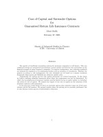
4
13579
λ = 1.0
λ = 0.6

Payoff at Maturity for a participating contract
6
The price of a contract having such a payoff is calculated in the following way:
V
0
= E
Q

e
−rT
L
T

, (5)
which leads to
V
0
= S
0
e
(g−r)T
+ λC
BS
0
(S
0
,S
0
e
gT

,r,σ,T) (6)
where C
BS
0
(S
0
,S
0
e
gT
,r,σ,T) represents the Black Scholes price of a European call option with
initial price of the underlying S
0
,astrikevalueS
0
e
gT
, interest rate r, volatility σ and maturity T.
At time t=0 the total premium received by the insurance company is P
0
= V
0
. Inadditionthe
shareholder injects a certain level of target capital TC
0
in order to guarantee the solvency. The
assumption of "true" guarantee implies that if at maturity TC
0
e
rT

is not enough then an additional
injection will be made.
The initial investment strategy is as follows:
- F
0
= S
0
is invested in the risky asset
- V
0
− F
0
= V
0
− S
0
is invested in the riskless asset
-TC
0
is invested in the riskless asset
The total value of the assets of the company at date t=0 is given by A
0
= V
0
+ TC
0
.
At maturity T, the value of the assets of the company is defined in the following way,
A
T

=(TC
0
+(V
0
− S
0
)) e
rT
+ S
T
. (7)
The benefits to be paid to the policyholder are given by
L
T
= S
0
e
gT
+ λM ax

0,S
T
− S
0
e
gT

. (8)
We assume that the target level of the ruin probability α, is defined by the shareholder at time
t=0. The target capital TC

0
is the minimum capital satisfying the following relation
P [A
T
<L
T
| Initial shareholder capital = TC
0
] 6 α. (9)
Assuming that the initial value of the shareholder’s capital is TC
0
, we can write
A
T
<L
T
⇔ (TC
0
+(V
0
− S
0
)) e
rT
+ S
T
<S
0
e
gT

+ λMax

0,S
T
− S
0
e
gT

but we also have
A
T
<L
T
⇔ A
T
<L
g
T
= S
0
e
gT
,.
because insolvency can occur if and only if the value of assets is lower than the value of the
guaranteed benefits.
Therefore
{A
T
<L

T
} =

(TC
0
+(V
0
− S
0
)) e
rT
+ S
T
<S
0
e
gT

and hence
P [A
T
<L
T
]=P
⎡
⎢
⎢
⎣
S
T

<

S
0
e
gT
− (TC
0
+(V
0
− S
0
)) e
rT


 
β
⎤
⎥
⎥
⎦
= P [S
T
<β] . (10)
The relation P [S
T
<β]=α will be satisfied if and only if
β = S
0

e
(µ−
σ
2
2
)T +σ
√
Tw
T
(11)
where w
T
= Φ
−1
(α) is the inverse of the standard normal distribution.
7
Therefore the initial target capital is given by
TC
0
=

S
0
e
gT
− β

e
−rT
− (V

0
− S
0
) . (12)
In this section we assumed that at maturity the shareholder will honour its obligations in any
situation, therefore the target capital has no importance from the policyholder’s point of view. The
contract is clearly defined; the only information important for the policyholder is the price. Here,
the target capital is only a requirement from the regulator and there is no additional cost associated.
The price of the contract is independent of the level of the target capital and therefore when the
pricing is performed there is no necessity to consider simultaneously the question of the minimum
capital requirement.
The non consideration of the default risk of the insurer within the pricing of a contract fairly
represents the common practice in the market. This practice results from the information asymmetry
existing between policyholders and shareholders.
2.3 The case of a conditional guarantee
Manyinsurancecompaniesaresetintheformofalimited liability company. For these companies,
in case of insolvency there is no obligation for the shareholders to inject additional capital.
By considering the default of the company, the payoff to the policyholder becomes
L
T
=

S
0
e
gT
+ λMax

0,S
T

− S
0
e
gT

if S
T
≥ β
A
T
=(TC
0
+(V
0
− S
0
)) e
rT
+ S
T
if S
T
<β
, (13)
where β defines the threshold value of the stock price indicating insolvency,
{S
T
<β} ⇔

A

T
<L
g
T
= S
0
e
gT

.
We can also write the payo ff in the following way,
L
T
= S
0
e
gT
+ λMax

0,S
T
− S
0
e
gT

· 1
{S
T
≥β}

+

(TC
0
+(V
0
− S
0
)) e
rT
+ S
T

· 1
{S
T
<β}
, (14)
or
L
T
= S
0
e
gT
· 1
{S
T
≥β}
+ λ(S

T
− S
0
e
gT
) · 1
{
S
T
≥Max
{
S
0
e
gT
,β
}}
+

(TC
0
+(V
0
− S
0
)) e
rT
+ S
T


· 1
{S
T
<β}
. (15)
0.5 1 1.5 2
0.6
0.8
1.2
1.4
1.6
1.8
Payoff at Maturity as a function of S
T
considering the default of the insurer
8
Comparing to the true guarantee case, the contract includes an additional put option in favour
of the company. Ignoring default implies an overpricing of the contract and results therefore in an
additional value creation for the shareholders.
The price of such contracts are calculated in the following way
V
0
= E
Q

e
−rT
L
T


(16)
which leads to
V
0
· e
rT
=S
0
e
gT
· Q [S
T
≥ β] − λS
0
e
gT
· Q

S
T
≥ Max

S
0
e
gT
,β

+λE
Q


S
T
· 1
{
S
T
≥Max
{
S
0
e
gT
,β
}}

+Q [S
T
<β] · (TC
0
+(V
0
− S
0
)) e
rT
+E
Q

S

T
· 1
{S
T
<β}

,
or
V
0
= S
0
e
(g−r)T
· N (d
2
) − λS
0
e
(g−r)T
· N (h
2
)+λS
0
· N (h
1
)
+(TC
0
+(V

0
− S
0
)) · N (−d
2
)+S
0
· N (−d
1
) , (17)
with
d
1
=
ln

S
0
β

+

r +
σ
2
2

T
σ
√

T
,d
2
= d
1
− σ
√
T (18)
and
h
1
=
ln

S
0
K

+

r +
σ
2
2

T
σ
√
T
,h

2
= h
1
− σ
√
T, K = Max

S
0
e
gT
,β

. (19)
The target capital is defined in a similar way as in the case of a "true" guarantee:
TC
0
=

S
0
e
gT
− β

e
−rT
− (V
0
− S

0
) . (20)
Replacing in the previous formula gives the following expression for the price of the contract:
V
0
= S
0
e
(g−r)T
· N (d
2
) − λe
(g−r)T
S
0
· N (h
2
)+λS
0
· N (h
1
)
+

S
0
e
gT
− β


e
−rT
· N (−d
2
)+S
0
· N (−d
1
) . (21)
When default is considered, the price of the contact depends directly on the value of the target
capital. Therefore, the pricing and the valuation of the target capital have to be solved simultane-
ously. The difference in price compared with the "true" guarantee case is a deduction of an amount
corresponding to the value of the right of the shareholder to not inject additional capital in the
company.
9
The following example shows the variation of the price of the contract and the target capital with
a change in the level of solvency α.
0.5 0.6 0.7 0.8 0.9
1
−α
0.2
0.4
0.6
0.8
1
8
__Price ,
−−
TC
<

Price and Target capital as function of 1-α,
S
0
=1,r=0.15,µ=0.17,g=0.08,σ=0.3,λ=0.95,T=1
The price of the contract and the target capital are increasing functions of the solvency level α.
We have lim
α→0
TC
0
(α)=+∞, but this convergence is slow due to the short-tail distribution of
the financial uncertainty W which is assumed to be normally distributed. The target capital is more
sensitive to the solvency level than the price is. The level of the solvency α will have an impact on
the payoff only when the stock price S
T
is in the critical region below β. The probability to be in this
critical region decreases with lower levels of α, this explains why the price is less sensitive than the
target capital.
We note also that the price of the contract is increasing with the level of the target capital. In
order to charge the policyholder with a maximum price, the company could be tempted to increase
indefinitely the level of the target capital. But as we will see in the next section, capital has a cost,
and the company can only have a limited resort to shareholders’ capital.
10
3CostofCapital
3.1 Incomplete markets and cost of capital
Insurance companies are required to maintain a minimum level of capital in order to satisfy the
solvency level. In the previous section this capital was represented by the target capital TC
0
. A
rational client will usually prefer to buy his contract from the more secure company. A simple way
for an insurance company to reduce its ruin probability is to increase the target capital to relatively

high levels. In practice we note that the access to equity capital has a cost. This cost is represented
by an extra return requirement by the shareholders on their invested assets. Part of this extra return
covers the risk that in case of default shareholders may not receive the full value of their investment.
Covering the default risk is equivalent to going back to the situation where pricing was performed
under the assumption of a "true" guarantee. In which case the value of the limited liability put
option was not deducted from the price of the contract. The practice shows that in addition to the
assumption of a "true" guarantee, the shareholders will still require an extra compensation. This
extra compensation is justified not only by capital costs resulting from market imperfections such
as frictional costs, double taxation or agency costs but mainly from the fact that the policyholder
agrees to pay more than the cost of the contract for the shareholder. We will summarize all these
extra compensations to the shareholder under the term of "cost of capital". And we consider the
cost of capital to be entirely explained by the risk aversion of the policyholder who can not access
or replicate the payoff of the contract outside the offer of the company. In such incomplete markets
there is usually no uniqueness of prices satisfying no-arbitrage conditions. The final prices will be
chosen by the insurance company according to the level of the competition in the market. For a new
contract, the insurer will fix the price at the highest level, and afterwards the price will be adjusted
with the inflow of new competitors.
Let us consider the following model to illustrate the incomplete market situation.
Let us assume that the insurance company wants to sell a contract with a term of one year (T=1).
We assume that this contract covers entirely a contingent claim C faced by the policyholder.
The preferences of the policyholders and the shareholders at time T are described by exponential
utilities with different absolute risk aversions α
P
and α
S
respectively.
Let u
P
be the utility function of the policyholder and u
S

the utility function of the shareholder.
u
P
(x)=1− e
−α
P
x
u
S
(x)=1− e
−α
S
x
And let W
P
and W
S
be the initial wealth of the policyholder and shareholder respectively.
We will de fine the price of the contract by the indifference price.
We assume that if the economic agents are not buying or selling the contract, then they will invest
their initial capital in the riskless asset and will wait to face the contingent claim at time t=T.
The indifference price p
S
for the shareholder is defined in the following way:
u
S
(W
S
(1 + r)) = E [u
S

((W
S
+ p
S
)(1+r) − C)] (22)
this gives,
p
S
=
1
α
S
(1 + r)
ln

E

e
α
S
C

(23)
p
S
is the minimal price at which the shareholder will accept to sell the contract.
The indifference price of the policyholder is defined as follows:
E [u
P
(W

P
(1 + r) − C)] = E [u
P
((W
P
− p
P
)(1+r)+C − C)] = u
P
((W
P
− p
P
)(1+r)) (24)
The first term can also be written as
E [u
P
(W
P
(1 + r) − C)] = E

1 − e
−α
P
(W
P
(1+r)−C)

=1− E


e
−α
P
(W
P
(1+r)−C)

=1− e
−α
P
(W
P
(1+r))
E

e
α
P
C

.
11