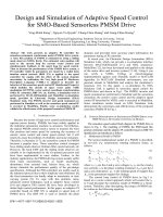
Design and Simulation of Adaptive Speed Control for SMO-Based Sensorless PMSM Drive

Design and Simulation of Adaptive Speed Control
for SMO-Based Sensorless PMSM Drive

Ying-Shieh Kung
1
, Nguyen Vu Quynh
2
, Chung-Chun Huang
3
and Liang-Chiao Huang
4


1,2
Department of Electrical Engineering, Southern Taiwan University, Taiwan
2
Department of Electrical Engineering, Lac Hong University, Vietnam
3,4
Green Energy and Environment Research Laboratories, Industrial Technology Research Institute, Taiwan


Abstract- The work presents an adaptive PI controller for
sensorless permanent synchronous motor (PMSM) drive system.
A rotor flux position of PMSM is estimated by using a sliding
mode observer (SMO), firstly. The estimated rotor position will
send to the current loop for current vector control and
simultaneously feedback to the speed loop for speed control.
Then to increase the performance of the PMSM drive system, a
PI controller which its parameters are tuned by a radial basis
function neural network (RBF NN) is applied to the speed
controller for coping with the effect of the system dynamic

uncertainty. In realization, the Very high speed IC Hardware
Description Language (VHDL) is adopted to describe the
behavior of the sensorless speed control IP (Intellectual Property)
which includes the circuits of space vector pulse width
modulation (SVPWM), vector control, coordinate transformation,
SMO, PI controller, RBF NN, etc. Further, a simulation work is
performed by MATLAB/Simulink and ModelSim co-simulation
mode, provided by Electronic Design Automation (EDA)
Simulator Link. The PMSM, inverter and speed command are
performed in Simulink as well as the sensorless speed control IP
is executed in ModelSim. Finally, some co-simulation results
validate the effectiveness of the proposed sensorless PMSM IP.
I. INTRODUCTION
Because the merits of high servo control performances and
superior power density, PMSMs has been widely applied in
the industrial automation machine as actuators. Nevertheless,
the typical PMSM control needs a sensor to measure the rotor
flux position and motor speed for ensuring the accuracy of
current vector control and motor speed control, but it will
relatively cause the problem of reliability and noise immunity.
Therefore, in literature [1-7], the sensorless control for PMSM
becomes a popular issue. Those sensorless control strategies
have sliding mode observer, Kalman filter, neural network, etc.
However, the back EMF and the sliding mode observer are
suitable to be implemented by the fix-pointed processor and
have been implemented in most studies. Further, in the
industry applications, the PMSM driving system usually suffer
from many uncertainties, such as model uncertainty,
disturbance from external load, friction force, etc. which
always diminish the performance quality of the pre-design

specification. Although the PID controllers are widely used in
the industrial process due to their simplicity and robustness [8],
the fixed parameters can hardly adapt to uncertainty or time
varying system [9]. To cope with this problem, many
advanced control techniques, such as adaptive fuzzy control
[10] and adaptive PID control [9] have been developed to
obtain high control performance. In this paper, an adaptive PI
controller based on RBF NN is adopted in speed loop of
PMSM drive. The RBF NN is used to identify the plant
dynamic and provided more accuracy plant information for
parameters tuning of PI controller.
In recent year, An Electronic Design Automation (EDA)
Simulator Link, which can provide a co-simulation interface
between MALTAB/Simulink [11] and HDL simulators-
ModelSim [12], has been developed and applied in the design
of the motor drive and inverter system [13-16]. Using it you
can verify a VHDL, Verilog, or mixed-language
implementation against your Simulink model or MATLAB
algorithm. In MATLAB/ Simulink environment, you can
generate stimuli to ModelSim and analyze the simulation’s
responses [11]. In this paper, a co-simulation by EDA
Simulator Link is applied to sensorless speed control for
PMSM drive and shown in Fig.1. The PMSM, inverter and
speed command are performed in Simulink and the sensorless
estimation, the current vector control and the adaptive speed
control IP described by VHDL code is executed in ModelSim.
Some simulation results based on EDA Simulator Link
demonstrate the correctness and effectiveness of the proposed
sensorless PMSM IP in Fig.1.
II. S

YSTEM DESCRIPTION OF SENSORLESS PMSM DRIVE AND
RBF NEURAL NETWORK CONTROLLER DESIGN
The sensorless speed control block diagram for PMSM drive is
shown in Fig. 1. The modeling of PMSM, the SMO-based flux
position estimation and the adaptive PI controller based on RBF NN
identification are introduced as follows:
A. Mathematical Model of PMSM
The typical mathematical model of a PMSM is described,
in two-axis d-q synchronous rotating reference frame, as
follows
d
d
q
d
q
ed
d
sd
L
i
L
L
i
L
r
dt
di
v
1



(1)
q
qq
eq
q
s
d
q
d
e
q
LL
K
i
L
r
i
L
L
dt
di
v
1


E


(2)

where v
d
, v
q
are the d and q axis voltages; i
d
, i
q
, are the d and q
axis currents, r
s
is the phase winding resistance; L
d
, L
q
are the d
and q axis inductance;
e

is the rotating speed of magnet flux;
E
K
is the permanent magnet flux linkage.
The current loop control of PMSM drive in Fig.1 is
based on a vector control approach which will control the i
d

to 0 and decouple the nonlinear model of PMSM to a linear
system. Therefore, after decoupling, the torque of PMSM can
be written as the following equation,

qtqEe
iKiK
P
T
4
3


(3)
978-1-4577-1967-7/12/$26.00 ©2011 IEEE


DC
Power
PMSM
Model
IGBT-based
Inverter
PWM1
PWM6
PWM2
PWM3
PWM4
PWM5
r

Flux angle
Transform.
r


SimuLink
A
B
C
External load
SVPWM
PI
0
*

d
i
q
i
d
i
Park Clark
Park
-1
Clark
-1
—
—
+
PI
1ref
v
3ref
v
2ref

v
q
v
d
v

v

v

i

i
*
q
i
+
a,b,c


,
d,q


,


,
d,q



,
a,b,c
Current
controller
a
i
b
i
c
i
Modify
sin /cos of
Flux angle
ee
ˆ
cos/
ˆ
sin


v

v

i

i
Rotor flux
position

estimation
e
ˆ

ModelSim
a
i
b
i
c
i
e

r

Current controllers and coordinate
transformation (CCCT)
*
r

r

ˆ
m

Reference
Model
(RM)
+
_

RBF
Neural Network
+
_
PI Controller
rbf

nn
e
Adjusting Mechanism
e
Jacobian
1
Z
2
Z
*
q
i
Speed loop
de
Speed
estimator
r

ˆ

Fig.1 The block diagram of adaptive speed control for sensorless PMSM drive

Considering the mechanical load, the overall dynamic

equation of PMSM drive system is obtained by
Lermrm
TTB
dt
d
J 

(4)
where T
e
is the motor torque, P is pole pairs, K
t
is torque
constant, J
m
is the inertial value, B
m
is damping ratio, T
L
is the
external torque,
r

is rotor speed.
B. Algorithm of the rotor flux position estimation
The block diagram to estimate the rotor flux position in
Fig.1 is constructed in Fig. 2 which consists of a sliding mode
observer (SMO), a bang-bang controller, a low-pass filter and
a position computation. The inputs in this block
are

)(),(),(),( nvnvnini

, and the output is
e

ˆ
. The
algorithm of the rotor flux position estimation is presented as
follows:
Step 1: Read the values of currents and voltages in

and

axis,
)(),(),(),( nvnvnini

, from CCCT in Fig.1.
Step 2: Estimate the estimated current by SMO








































)(
ˆ
)(

ˆ
)(
)(
)(
ˆ
)(
ˆ
0
0
)1(
ˆ
)1(
ˆ
ne
ne
nv
nv
ni
ni
ni
ni












(5)
where
s
s
T
L
r
e


,
)1(
1

s
s
T
L
r
s
e
r




and
s

T
is the sampling
time.
Step 3: Calculate the current error by
)()(
ˆ
)(
~
ninini


and
)()(
ˆ
)(
~
ninini


(6)
Step 4: Obtain the Z gain of the current observer
)
)(
~
)(
~
(*
)(
)(
)(

















ni
ni
signk
nz
nz
nZ




(7)
Step 5: Estimate the EMF

























)(
ˆ
)(
)(
ˆ
)(
2
)(

ˆ
)(
ˆ
)1(
ˆ
)1(
ˆ
0
nenz
nenz
f
ne
ne
ne
ne







(8)
Step 6: Obtain the estimated rotor position
)
)(
ˆ
)(
ˆ
(tan)(

ˆ
1
ne
ne
n
e





(9)
then set n=n+1 and back to Step 1.
Sliding mode
observer
—
+
—
+
Bang-bang
controller
Low-pass
filter
Flux angle
computation









v
v








i
i








i
ˆ
i










z
z








e
ˆ
e
ˆ
e
ˆ

Rotor position estimation

Fig.2 Rotor flux position estimation based on SMO
C. Adaptive PI controller using RBF NN
Adaptive PI controller in Fig.1 includes a PI controller, a
reference model and a RBF NN for system identification. The
detailed descriptions of those components are presented as
follows.

(1) PI controller
In Fig. 1, digital PI controllers are presented in the speed
loop of PMSM and the formulations are as follows.
)k(
ˆ
)k()k(e
rm




(10)
)k(eK)k(u
pp

(11)
)1()1())1()2((
))1()1(()1()(
1
22





keKku kekEK
kejeKjeKku
iii
k
j

i
k
j
ii
(12)
)1()1()()()()(
*
 keKkukeKkukuki
iipipq
(13)
with




1
2
)1()(
k
j
jekE
and
)2()1(  kEKku
ii
. Besides, where
r
ˆ

,
m


,
e
are the estimated rotor speed, the output of
reference model and the error, respectively. The
p
K
,
i
K
are P
controller gain and
I controller gain, respectively. The
)k(u
p
,
)k(u
i
,
)k(i
*
q
are the output of P controller only, I
controller only and the PI controller, respectively.
(2) Radial basis function neural network (RBF NN)
Fig. 3 shows the RBF NN which is three-layer architecture
by an input layer, a single layer of nonlinear processing
neurons and an output layer. The RBF NN has three inputs
by
)k(i

*
q
,
)1(
ˆ
k
r

,
)2(
ˆ
k
r

and its vector form is represented
by
T
rrq
kkkiX )]2(
ˆ
),1(
ˆ
),([
*


(14)
Furthermore, the multivariate Gaussian function is used as the
activated function in hidden layer of RBF NN, and its
formulation is shown as follows.

pr
cX
h
r
r
r
, 4,3,2,1),
2
exp(
2
2




(15)
where
p is the number of neuron in hidden layer,
T
rrrr
cccc ],,[
321

and
r

respectively denote center and
node variance of
r
th

neuron, and
r
cX 
is the norm value
which is measured by the inputs and the node center at each
neuron. And the network output in Fig. 3 can be written as



p
r
rrrbf
hw
1

(16)
where
rbf

is the output value;
r
w
and
r
h
are the weight and
output of
r
th
neuron, respectively.

Define the cost function as follows.
22
2
1
)
ˆ
(
2
1
nnrrbf
eJ 

(17)
Then, according to the gradient descent method, the learning
algorithm of weights, node center and variance are as follows:
)()()()1( khkekwkw
rnnrr


(18)
)(
)()(
)()()()()1(
2
k
kckX
khkwkekckc
r
rss
rrnnrsrs





(19)
)(
)()(
)()()()()1(
3
2
k
kckX
khkwkekk
r
r
rrnnrr




(20)
where
r=1,2, p, s=1,2,3 and

is a learning rate. Further, the
Jacobian transformation can be derived from Fig.3 and (16)
and it is










p
r
r
qr
rr
q
rbf
q
r
kic
hw
ii
1
2
*
1
**
)(
ˆ



(21)


)(
*
ki
q
)1(
ˆ
k
r

)2(
ˆ
k
r

rbf

1
w
2
w
1
h
p
w
2
h
p
h
Input layer
Hidden layer

Output layer
)(
ˆ
k
r

nn
e
+
-

Fig.3 The architecture of RBF NN
(3) Reference Model (RM):
Second order system is usually considered to taken as the
RM in the adaptive control system
22
2
2
nn
n
*
r
m
ss)s(
)s(







(22)
where
n

is natural frequency and

is damping ratio.
Furthermore, applying the bilinear transformation, (22) can be
transformed to a discrete model by
2
2
1
1
2
2
1
10
1
1
1







zz
zz

)z(
)z(
*
r
m




(23)
and the difference equation is written as.
)2()1(
)()2()1()(
*
2
*
1
*
021


kk
kkkk
rr
rmmm


(24)
(4)
Adjusting Mechanism of PI Controller

The gradient descent method is used to derive the tuning
law of PI controller in Fig. 1. The adjusting mechanism is to
minimize the square error between the rotor speed and the
output of the reference model. The instantaneous cost function
is firstly defined by
222
2
1
2
1
2
1
)
ˆ
()( e J
rmrme


(25)
and the parameters of PI controller are adjusted according to
p
e
p
e
p
K
J
K
J
K








(26)
And

i
e
i
e
i
K
J
K
J
K







(27)
where


represents learning rate. Secondly, the chain rule is
used, and the partial differential equation for
e
J
in (26) and
(27) can be written as
p
*
q
*
q
r
r
e
p
e
K
i
i
e
e
J
K
J














(28)
and
i
*
q
*
q
r
r
e
i
e
K
i
i
e
e
J
K
J














(29)
Further, from (10), (13), (25) and
rr


ˆ

, we can get
e
e
J
e



(30)
1






rr
ˆ
ee

(31)
)k(e
K
)k(i
p
*
q



(32)
)1()1()2(
)(
*



kEkekE
K
ki
i
q
(33)
Therefore, substituting (30)~(33) and (21) into (28) and (29),

the parameters of PI controller in (26) and (27) can be adjusted
by the following expression.
2
1
1
2
r
*
qr
p
r
rrp
)k(ic
hw)k(e )k(K






(34)
2
*
1
1
)(
)1()()(
r
qr
p

r
rri
kic
hwkEke kK






(35)
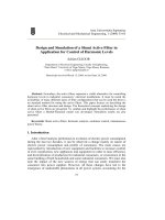
III. SIMULINK/MODELSIM CO-SIMULATION OF SENSORLESS
SPEED CONTROL FOR PMSM DRIVE
In Fig.1, it shows the sensorless speed control block
diagram for PMSM drive and its Simulink/ModelSim co-
simulation architecture is presented in Fig.4. The PMSM,
IGBT-based inverter and speed command are performed in
Simulink, and the sensorless speed controller described by
VHDL code is executed in ModelSim with three works., The
work-1 to work-3 of ModelSim in Fig.4 respectively performs
the function of speed estimation and speed loop adaptive PI
controller, the function of current controller and coordinate
transformation (CCCT) and SVPWM, and the function of
SMO-based rotor flux position estimation. The VHDL is used
to describe the works in ModelSim. In current loop of PMSM
drive, the sampling frequency is designed with 16kHz, and
those in speed loop is 2kHz. The clocks with 20ns and 80ns
periods are sent to work-1 and work3 of ModelSim.
A finite state machine (FSM) is employed to model the
adaptive PI controller and SMO which are shown in Fig.5 and

Fig.6, respectively.
In Fig.5, it manipulates 81 steps machine to
carry out the overall computations of an adaptive PI controller.
The steps s
0
~s
5
execute the reference model output; step s
6
perform the computation of speed error; steps s
7
~s
10
execute
the PI controller; steps s
11
~s
74
describe the RBF NN and
computation of Jacobian value and s
75
~s
80
execute the PI gain
tuning.
The data format adopts 16-bit (Q15) with signed
representation. The components of multiplier and adder use
Altera LPM (Library Parameterized Modules) standard and its
computation can be completed within 20ns. To prevent the
numerical overflow condition occurred, the executing time at

each step is designed with 80ns; therefore, in Fig.5, total 81
steps need 6.48
s. Further, In Fig.6, it manipulates 36 steps
machine to carry out the overall computations.
The steps s
0
~s
8

execute the estimation of current value; steps s
9
~s
10
compute
the current error; s
11
is the bang-bang control; s
12
~s
15
describe
the computation of EMF and s
16
~s
35
perform the computation
of the rotor position.
The data format adopts 12-bit (Q11) with
signed representation. The components of multiplier and adder
use Altera LPM standard but the component performing the

arctan function is developed ourselves. The executing time at
each step is designed with 80ns; therefore total 36 steps need
2.88
s. In Fig.4 the circuit design of CCCT and SVPWM in
work-2 of ModelSim are not shown here. The FPGA (Altera)
resource usages of work-1 to work-3 of ModelSim in Fig.4 are
8,942 LEs (Logic Elements) and 0RAM bits; 2,085 LEs and
24,576 RAM bits; 1,151LEs and 49,152 RAM bits,
respectively.
IV.
CO-SIMULATION BASED ON EDA SIMULATOR LINK
Based on EDA simulator link, the simulation architecture
for the proposed sensorless PMSM adaptive speed control
system is presented in Fig.4. The ModelSim performs the
function of adaptive PI controller, SMO and current vector
controller which is described using VHDL code. In the
Simulink, the SimPowerSystem blockset can provide the
components of PMSM and the inverter and it also can
generate stimuli to ModelSim and analyze the simulation’s
responses The designed PMSM parameters applied in
simulation of Fig.4 are that pole pairs is 4, stator phase
resistance is 1.3
, stator inductance is 6.3mH, inertia is
J=0.000108 kg*m
2
and friction factor is F=0.0013 N*m*s.
(work-2)
(work-1)
(work-3)

Fig.4 The Simulink/ModelSim co-simulation architecture for sensorless speed control of PMSM drive
x
x
+
x
+
x
s
0
s
1
s
2
s
3
s
4
s
5
x
+
-
+
-
s
6
+
-
+
s

7
)(
*
k
r

)1( k
m

)1( kE
0
a
1
a
2
a
1
b
2
b
s
8
Computation of the reference model output
Computation of the rotor speed
error and error change
s
11
~s
72
s

73
s
75
s
76
s
78
s
79
s
77
s
80
Computation of RBF NN and Jocobian
s
9
s
10
)(ke
)1(
*
k
r

)2(
*
k
r

)2( k

m

)(k
m

)(
ˆ
k
r

x
p
k
x
i
k
)(ke
+
)(ku
i
)1( ku
i
+
)(ku
p
PI controller
*
q
i
)(

*
ki
q
)(
ˆ
k
r

)1(
ˆ
k
r

Neuro-1
computation
Neuro-2
computation
Neuro-3
computation
+
out1
out2
out3
J1
J2
J3
+
+
rbf


+
Jaco
s
74
x
)(ke

x
Je
x
+
)1( kk
p
)(kk
p
x
)1( kE
+
)1( kk
i
)(kk
i
Tuning of the PI controller gains
)(kE

Fig. 5 State diagram of an FSM for describing the adaptive PI controller
+
x
s
0

s
1
s
2
s
3
s
4
)n(v

Estimation of the current values
s
10

s
11
)(
ˆ
ne

x

)n(i
ˆ

+
)n(i
ˆ
1


+ x
s
5
s
6
s
7
s
8
s
9
)n(v

)n(e
ˆ

x
)n(i
ˆ

+
)n(i
ˆ
1

-
+
)n(i

-

)n(i
ˆ

)n(i
~

+
)n(i

-
)n(i
ˆ




Y
N
k)n(z


k)n(z 


Y
N
k)n(z 

k)n(z 


x
s
12
s
13
s
14
s
15
s
24
)n(z

0
2 f

)n(e
ˆ

s
34
-
+
+
)n(e
ˆ

)n(e
ˆ
1


x
)n(z

)n(e
ˆ

-
+
+
)n(e
ˆ

)n(e
ˆ
1

e

ˆ
)n(i
~


)n(e
ˆ
)n(e
ˆ




s
16
s
23
-
tan
-1
atan2
s
35
Computation of
current errors
Bang-bang control
Estimation of the EMF
Computation of the rotor position
Table
s
17
-
0
2 f


Fig.6 State diagram of an FSM for describing the SMO-based rotor position
estimation algorithm
In the simulation of sensorless PMSM drive, rotor
position estimation based on SMO is firstly evaluated.
Three kinds of PMSM running speed at 500rpm, 1000rpm
and 1500 rpm are tested and its simulation results of the real

and estimated rotor flux position are presented in Fig.7. It
shows that the response of the estimated rotor flux position
e

ˆ
can follow with the actual rotor flux position
e

.
Secondly, the performance of adaptive PI control using RBF
NN identification is verified. Two tested cases are
considered under different PMSM parameters, in which
Case 1: (Normal-load condition)
J=0.000108, F=0.0013 (36)
Case II: (Heavy-load condition)
J=0.000108*3, F=0.0013*3 (37)
When speed loop adopts PI controller only (K
p
=1500, K
i
=30)
and sensorless PMSM drive runs at the normal-load
condition and at 0~1500 rpm speed range, the simulation
result of the step speed response with no overshoot and
0.25s rising time characteristics is shown in Fig.8. But when
the running condition is changed to the heavy-load condition
and speed range is operated from 0~800 rpm, the step speed
response become worse with a little overshoot and
sluggishness in Fig.9. It demonstrates that although the
sensorless control based on SMO in PMSM drive can give a

good speed tracking, it is still easily affected by external
load variation. To cope with this problem, an adaptive PI
control with RBF NN identification is adopted in Fig.1. The
RBF NN will identify the plant dynamic and provide more
accuracy plant information for parameters tuning of PI
controller. Figures 10~11 show the simulation results while
it uses the proposed adaptive PI control in sensorless PMSM
drive. In this two Figs., the K
p
and K
i
are respectively set
with 1500 (Q15 format) and 30 (Q15 format) at the initial
condition; then K
p
and K
i
will be tuned to the adequate
values to let the rotor response can follow the output of the
reference model. Compare with Fig. 9, the result of Fig. 11
(c) shows an apparent improvement which the rotor speed
can follow the output of RM after 1 sec. It also present that
the proposed adaptive controller can enhance the robustness
in sensorless PMSM drive.
V.
CONCLUSIONS
This study has been presented an adaptive speed
control in SMO-based sensorless PMSM drive and
successfully demonstrated its performance through co-
simulation by using Simulink and ModelSim. In realization

aspect, the VHDL is used to describe the behavior of the
SMO estimator and the adaptive PI controller algorithm, and
FSM method is applied to reduce the FPGA resource usage.
In computational power aspect, the operation time to
complete the computation of the SMO estimator and the
adaptive PI controller algorithm are only 2.88
s and 6.48s,
respectively. In controller performance aspect, some
simulation results show that the proposed adaptive PI
controller for sensorless PMSM is effectiveness and
robustness. After confirming the effective of VHDL code in
adaptive PI control IP and rotor position estimation IP, the
codes can be directly downloaded to FPGA for the use in
sensorless PMSM drive.



Fig. 7 Real rotor flux angle (
e

) and estimated rotor flux angle (
e

ˆ
) under
PMSM speed running at (a)500rmp, (b)1000rpm and (c)1500rpm
0 0.5 1 1.5 2 2.5 3
0
500
1000

1500
2000
Time (s)
Speed
command
Rotor
speed
Reference
model
Speed (rpm)

Fig. 8 Step speed response using PI controller only with K
p
=1500, K
i
=30
while sensorless PMSM operated at normal load condition
0 0.5 1 1.5 2 2.5 3
0
200
400
600
800
1000
Time (s)
Speed
command
Rotor
speed
Reference

model
Speed (rpm)

Fig. 9 Step speed response using PI controller only with K
p
=1500, K
i
=30
while sensorless PMSM operated at heavy load condition
0 0.5 1 1.5 2 2.5 3
0
10
20
30
40
50
60
0 0.5 1 1.5 2 2.5 3
0
200
400
600
800
1000
Time (s)
0 0.5 1 1.5 2 2.5 3
0
1000
2000
3000

4000
5000
Speed
command
Reference
model
Rotor
speed
(a)
(b)
(c)
Speed (rpm) K
i
gain
K
p
gain

Fig. 10 Step speed response using adaptive PI controller while sensorless
PMSM operated at normal load condition. (a) K
p
variation (b) K
i

variation (c) speed response
0 0.5 1 1.5 2 2.5 3
0
1000
2000
3000

4000
5000
Time (s)
0 0.5 1 1.5 2 2.5 3
0
10
20
30
40
50
60
70
Time (s)
0 0.5 1 1.5 2 2.5 3
0
200
400
600
800
1000
Time (s)
Speed
command
Rotor
speed
Reference
model
(a)
(b)
(c)

Speed (rpm) K
i
gain
K
p
gain

Fig 11. Step speed response using adaptive PI controller while sensorless
PMSM operated at heavy load condition. (a) K
p
variation (b) K
i

variation (c) speed response.
ACKNOWLEDGMENT
The financial support provided by Bureau of Energy is
gratefully acknowledged.
REFERENCE
[1] Y.S, Han, J.S. Choi and Y.S. Kim, “Sensorless PMSM Drive with
Sliding Mode Control Based Adaptive Speed and Stator Resistance
Estimator,”
IEEE Trans. on Magnetics, vol. 36, no. 5, pp.3588~3591,
Sep. 2000.
[2]
M. Ezzat, J.d. Leon, N. Gonzalez and A. Glumineau, “Sensorless
Speed Control of Permanent Magnet Synchronous Motor by using
Sliding Mode Observer,”
in Proceedings of 2010 11th International
Workshop on Variable Structure Systems
, pp.227~232, June 26 - 28,

2010.
[3]
V.D. Colli, R.D. Stefano and F. Marignetti, “A System-on-Chip
Sensorless Control for a Permanent-Magnet Synchronous Motor,”
IEEE Trans. on Indus. Electron., vol. 57, no. 11, pp.3822~3829, Nov.
2010.
[4]
T.D. Batzel and K.Y. Lee, “An Approach to Sensorless Operation of
the Permanent-Magnet Synchronous Motor Using Diagonally
Recurrent Neural Networks,”
IEEE Trans. on Energy Conversion, vol.
18, no. 1, pp.100~106, March 2003.
[5]
P. Borsje, T.F Chan, Y.K. Wong, and S.L. Ho, “A Comparative Study
of Kalman Filtering for Sensorless Control of a Permanent-Magnet
Synchronous Motor Drive,”
in Proceedings of IEEE International
Conference on Electric Machines and Drives,
pp.815~822, 2005.
[6]
M. C. Huang, A. J. Moses and F. Anayi and X. G. Yao, “Reduced-
Order Linear Kalman Filter (RLKF) Theory in Application of
Sensorless Control for Permanent Magnet Synchronous
Motor(PMSM),”
in Proceedings of IEEE Conference on Industrial
Electronics and Applications
, pp.1~6, 2006.
[7]
L. Idkhajine and E. Monmasson, “Design methodology for complex
FPGA-based controllers –Application to an EKF Sensorless AC

Drive,”
in Proceedings of International Conference on Electrical
Machines
(ICEM), pp. 1-6, 2010.
[8]
K.J. Astrom, T. Hangglund, C.C. Hang and W,K, Ho, “Automatic
Tuning and Adaptation for PID Controller – A survey,”
IFAC J. Contr.
Eng. Practice
, vol. 1, no.4, pp.699-714, 1993.
[9]
M.G. Zhang, X.G. Wang and M.G. Liu, “Adaptive PID Control based
on RBF neural network identification,” in Proc. of the
IEEE
International Conference on
Tools with Artificial Intelligence, Nov.
14-16, 2005.
[10]
Y.S. Kung and M.H. Tsai, “FPGA-based Speed Control IC for PMSM
Drive with Adaptive Fuzzy Control”,
IEEE Trans. on Power
Electronics
, vol. 22, no. 6, pp. 2476-2486, Nov. 2007.
[11]
The Mathworks, Matlab/Simulink Users Guide, Application Program
Interface Guide
, 2004
[12]
Modeltech, ModelSim Reference Manual, 2004.
[13]

M.F. Tsai, Tran Phu Quy, B.F. Wu, and C.S. Tseng, “Model
Construction and Verification of a BLDC Motor Using
MATLAB/SIMULINK and FPGA Control,”
in Proceedings of the
2011 6th IEEE Conference on Industrial Electronics and Applications,
pp.1797-1802, 2011.
[14]
Y.S. Kung, V.Q. Nguyen, Chung-Chun Huang and L.C. Huang,
“Simulink/ModelSim Co-Simulation of Sensorless PMSM Speed
Controller,”
in Proceedings of the 2011 IEEE Symposium on
Industrial Electronics and Applications (ISIEA 2011)
, pp.24-29, 2011.
[15]
D. Feng, L. Yan; L. Xu and W. Li “Implement of Digital PID
Controller Based on FPGA and the System Co-simulation,”
in
Proceedings of
the 2011 International Conference on Instrumentation,
Measurement, Computer, Communication and Control
, pp.921-924,
2011.
[16]
M.F. Tsai, F. J. Ke, L.C. Hsiao, and J.K. Wang, “Design of a Digital
Control IC of a Current Source Based on a Three-Phase Controlled
Rectifier,”
in Proceedings of the IEEE 6th International Power
Electronics and Motion Control Conference (IPEMC
), pp.337-343,
2009.