Proceedings VCM 2012 24 a simple walking control method for biped robot

Tuyển tập công trình Hội nghị Cơ điện tử toàn quốc lần thứ 6 169


Mã bài: 39
A Simple Walking Control Method for Biped Robot
with Stable Gait
Tran Dinh Huy, Nguyen Thanh Phuong, Ho Dac Loc, *Tran Quang Thuan
Ho Chi Minh City University of Technology, Vietnam
* Posts and Telecommunications Institute of Technology branch Hochiminh city
e-Mail:
Abstract:
This paper proposes a simple walking control method for a 10 degree of freedom (DOF) biped robot with
stable and human-like walking using simple hardware configuration. The biped robot is modeled as a 3D
inverted pendulum. From dynamic model of the 3D inverted pendulum and under the assumption that center of
mass (COM) of the biped robot moves on a horizontal constraint plane, zero moment point (ZMP) equations of
the biped robot depending on the coordinate of the center of the pelvis link obtained from the dynamic model
of the biped robot are given based on the D’Alembert’s principle. A walking pattern is generated based on
ZMP tracking control systems that are constructed to track the ZMP of the biped robot to zigzag ZMP
reference trajectory decided by the footprint of the biped robot. An optimal tracking controller is designed to
control the ZMP tracking control system. When the ZMP of the biped robot is controlled to track the x and y
ZMP reference trajectories that always locates the ZMP of the biped robot inside stable region known as area
of the footprint, a trajectory of the COM is generated as a stable walking pattern of the biped robot. Based on
the stable walking pattern of the biped robot, a stable walking control method of the biped robot is proposed by
using the inverse kinematics. From the trajectory of the COM of the biped robot and an arc reference input of
the swinging leg, the inverse kinematics solved by the solid geometry method is used to compute the angles of
each joint of the biped robot. These angles are used as references angles. Because the reference angles of the
biped robot are computed from the stable walking pattern of the biped robot, the walking of the biped robot is
stable if the angles of each joint of the biped robot are controlled to track those reference angles. The stable
walking control method of the biped robot is implemented by simple hardware using PIC18F4431 and
dsPIC30F6014. The simulation and experimental results show the effectiveness of this proposed control
method

Keywords: Optimal Tracking Controller; ZMP Tracking Control System; Biped Robot.

1. Introduction
Research on humanoid robots and biped robots
locomotion is currently one of the most exciting
topics in the field of robotics and there exist many
ongoing projects. Although some of those works
have already demonstrated very reliable dynamic
biped walking [11], it is still important to
understand the theoretical background of the biped
robot. The biped robot performs its locomotion
relatively to the ground while it is keeping its
balance and not falling down. Since there is no
base link fixed on the ground or the base, the gait
planning and control of the biped robot is very
important but difficult. Up so far, numerous
approaches have been proposed. The common
method of these numerous approaches is to restrict
zero moment point (ZMP) within a stable region to
protect the biped robot from falling down [2].
In the recent years, a great amount of scientific
and engineering research has been devoted to the
development of legged robots able to attain gait
patterns more or less similar to human beings.
Towards this objective, many scientific papers
have been published, focusing on different aspects
of the problem. Sunil, Agrawal and Abbas [3]
proposed motion control of a novel planar biped
with nearly linear dynamics. They introduced a
biped robot that the model was nearly linear. The

motion control for trajectory following used
nonlinear control method. Park [4] proposed
impedance control for biped robot locomotion so
that both legs of the biped robot were controlled
by the impedance control, where the desired
impedance at the hip and the swing foot was
specified. Huang and Yoshihiko [5] introduced
sensory reflex control for humanoid walking so
that the walking control consisted of a feedforward
dynamic pattern and a feedback sensory reflex. In
these papers, the moving of the body of the robot
was assumed to be only on the sagittal plane. The
170 Tran Dinh Huy, Nguyen Thanh Phuong, Ho Dac Loc, Tran Quang Thuan


VCM2012
biped robot was controlled based on the dynamic
model. The ZMP of the biped robot was measured
by sensors so that the structure of the biped robot
was complex and the biped robot required a high
speed controller hardware system.
This paper presents a stable walking control of a
biped robot by using the inverse kinematics with
simple hardware configuration based on the
walking pattern which is generated by ZMP
tracking control systems. The robot’s body can
move on the sagittal and the lateral planes.
Furthermore, the walking pattern is generated
based on the ZMP of the biped robot so that the
stability of the biped robot during walking or

running is guaranteed without the sensor system to
measure the ZMP of the biped robot. In addition,
the simple inverse kinematics using the solid
geometry is used to obtain angles of each joints of
the biped robot based on the stable walking
pattern. The biped robot is modeled as a 3D
inverted pendulum [1]. The ZMP tracking control
system is constructed based on the ZMP equations
to generate a trajectory of COM. A continuous
time optimal tracking controller is also designed to
control the ZMP tracking control system. From the
trajectory of the COM, the inverse kinematics of
the biped robot is solved by the solid geometry
method to obtain angles of each joint of the biped
robot. It is used to control walking of the biped
robot.
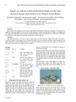
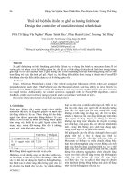
2. Mathematic Model Of The Biped Robot
A new biped robot developed in this paper has 10
DOF as shown in Fig. 1.

Fig. 1 Configuration of 10 DOF biped robot.
The biped robot consists of five links that are one
torso, two links in each leg those are upper link
and lower link, and two feet. The two legs of the
biped robot are connected with torso via two DOF
rotating joints which are called hip joints. Hip
joints can rotate the legs in the angles

5
for right

leg and

7
for left leg on sagittal plane, and in the
angles

4
for right leg and

6
for left leg on in
frontal plane. The upper links are connected with
lower links via one DOF rotating joints those are
called knee joints which can rotate on sagittal
plane. The lower links of legs are connected with
feet via two DOF of ankle joints. The ankle joints
can rotate the feet in angle

1
(for right leg) and

10

(for left leg) on the sigattal plane, and in angle

2

for left leg and

9

for right leg on the in frontal
plane. The rotating joints are considered to be
friction-free and each one is driven by one DC
motor.
2.1 Kinematics model of biped robot
It is assumed that the soles of robot do not slip. In
the world coordinate system 
w
which the origin is
set on the ground, the coordinate of the center of
the pelvis link and the ankle of swing leg can be
expressed as follows:


13211bc
sinlsinlxx


(1)


 
42
3
213221bc
cos
2
l
sincoslsinlyy





(2)
   
42
3
2132
211bc
sin
2
l
coscosl
coscoslzz




(3)
In choosing Cartesian coordinate 
a
which the
origin is taken on the ankle, position of the center
of the pelvis link is expressed as follows:


13211ca
sinlsinlx



(4)


 
42
3
213221ca
cos
2
l
sincoslsinly




(5)
   
42
3
2132
211ca
sin
2
l
coscosl
coscoslz





(6)
where, x
ca
, y
ca
, z
ca
are position of the center of the
pelvis link in 
a
.
Similarly, position of the ankle joint of swing leg
is expressed in the coordinate system 
h
which the
origin is taken on the center of pelvis link as:


78172eh
sinlsinlx


(7)
 
678162
3
eh
sincoslsinl
2
l

y


(8)


6781762eh
coscoslcoscoslz


(9)
It is assumed that the center of mass of each link is
concentrated on the tip of the link and the initial
z

x

y

Knee
a
b
3

8

1

2


5

4

10

9

6

7

A
nkle
Pelvis
Torso
z
h

x
h

y
h

z
a

x
a

y
a

l
2

l
1

0
B
2
(x
b
,y
b
,z
b
)

K
1

B
2

B
1

C
B

K
E
C(x
c
,y
c
,z
c
)
Foot
Hip
Tuyển tập công trình Hội nghị Cơ điện tử toàn quốc lần thứ 6 171


Mã bài: 39
position is located at the origin of the 
w
. This
means that x
b
= 0 and y
b
= 0.
The COM of the robot can be obtained as follows:
e43c21b
ee4433cc2211bb
com

mmmmmmm
xmxmxmxmxmxmxm
x



(10)
e43c21b
ee4433cc2211bb
com
mmmmmmm
ymymymymymymym
y



(11)
e43c21b
ee4433cc2211bb
com
mmmmmmm
zmzmzmzmzmzmzm
z



(12)
where (x
b
, y

b
, z
b
) and (x
e
, y
e
, z
e
) are coordinates of
the ankle joints B
2
and E, (x
1
, y
1
, z
1
) and (x
4
, y
4
, z
4
)
are coordinates of the knee joints B
1
and K
1
, (x

2
,
y
2
, z
2
) and (x
3
, y
3
, z
3
) are coordinate of the hip
joints B and K, (x
c
, y
c
, z
c
) is coordinate of the
center of pelvis link C, m
b
and m
e
are the mass of
ankle joints B
2
and E, m
1
and m

4
are the mass of
knee joints B
1
and K
1
, m
2
and m
3
are the mass of
hip joints B and K, and m
c
is the mass of the center
of pelvis link C.
If the mass of links of legs is negligible compared
with mass of the trunk, Eqs. (1)~(3) can be
rewritten as follows:
ccom
xx 
(13)
ccom
yy

(14)
ccom
zz 
(15)
It means that the COM is concentrated on the
center of the pelvis link.

In this paper, Eqs. (13)~(15) are used.
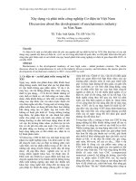
2.2 Dynamic model of biped robot
When the biped robot is supported by one leg, the
dynamics of the robot can be approximated by a
simple 3D inverted pendulum whose leg is the foot
of biped robot and head is COM of biped robot as
shown in Fig. 2.

Fig. 2 Three dimension inverted pendulum.
The length of inverted pendulum r is able to be
expanded or contracted. The position of the mass
point p = [x
ca
, y
ca
, z
ca
]
T
can be uniquely specified
by a set of state variable q = [

r
,

p
, r]
T
as follows
[1]:

p
rS
p
sinrx
ca


(16)
rrca
rSsinry 

(17)
rDsinsin1rz
p
2
r
2
ca


(18)

[

r
,

p
, f]

T
is defined as actuator torques and force
associated with the variables [

r
,

p
, r]
T
. The
Lagrangian of the 3D inverted pendulum is
ca
2
ca
2
ca
2
ca
mgz)zyx(m
2
1
L 


(19)
where m is the total mass of the biped robot, g is
the gravity acceleration.
Based on the Largange’s equation, the dynamics
of 3D inverted pendulum can be obtained in the

Cartesian coordinate as follows:

































































D
D
SrC
D
SrC
mg
fz
y
x
DSS
D
SrC
0rC
D
SrC
rC0
m
pp
rr
p
r
ca
ca
ca
rp
pp

p
rr
r





(20)
Multiplying the first row of the Eq. (20) by D/C
r

yields
 
rr
r
carca
mgrS
C
D
zrSyrDm 



(21)
Substituting Eqs. (16) and (17) into Eq. (21), the
dynamics equation of inverted pendulum along y
ca

axis can be obtained as



caxcacacaca
mgyzyyzm 





(22)
where
r
C
D
x


is the torque around x axis.
Using similar procedure, the dynamics equation of
inverted pendulum along x
ca
axis can be derived
from the second row of the Eq. (20) as


caycacacaca
mgxzxxzm 






(23)
where
p
p
y
C
D


is the torque around y axis.
The motions of the point mass of inverted
pendulum are assumed to be constrained on the
plane whose normal vector is [k
x
, k
y
, -1]
T
and z
intersection is z
c
. The equation of the plane can be
expressed as
ccaycaxca
zykxkz 
(24)
where k
x

, k
y
, z
c
are constant.
Second order derivative of Eq. (31) are
caycaxca
ykxkz








(25)
x
a

y
a

z
a


P



r


r


P

r

f
P

f
r

0

p
f

172 Tran Dinh Huy, Nguyen Thanh Phuong, Ho Dac Loc, Tran Quang Thuan


VCM2012
Substituting Eqs. (24) and (25) into Eqs. (22) and
(23), the equation of motion of 3D inverted
pendulum under constraint can be expressed as
 
x

c
cacacaca
c
x
ca
c
ca
mz
1
yxyx
z
k
y
z
g
y



(26)
 
y
c
cacacaca
c
y
ca
c
ca
mz

1
yxyx
z
k
x
z
g
x



(27)
It is assumed that the biped robot walks on the flat
floor and horizontal plane. In this case, k
x
and k
y

are set to zero. It means that the mass point of
inverted pendulum moves on a horizontal plane
with the height z
ca
= z
c
. Eqs. (26) and (27) can be
rewritten as
x
c
ca
c

ca
mz
1
y
z
g
y



(28)
y
c
ca
c
ca
mz
1
x
z
g
x



(29)
When inverted pendulum moves on the horizontal
plane, the dynamic equation along the x
ca
axis and

y
ca
axis are independent and linear differential
equations[1].
(x
zmp
, y
zmp
) is defined as location of ZMP on the
floor as shown in Fig. 3.
ZMP is such a point where the net support torque
from floor about x
ca
axis and y
ca
axis is zero. From
D’Alembert’s principle, ZMP of inverted
pendulum under constraint can be expressed as
ca
c
cazmp
x
g
z
xx


(30)
ca
c

cazmp
y
g
z
yy

 (31)







Fig. 3 ZMP of inverted pendulum.

Eq. (30) shows that position of ZMP along x
ca
axis
is linear differential equation and it depends only
on the position of mass point along x
ca
axis.
Similarly, position of ZMP along y
ca
axis do not
depend on x
ca
but only on y
ca

axis.


3. WALKING PATTERN GENERATION
The objective of controlling the biped robot is to
realize a stable walking or running. The stable
walking or running of the biped robot depends on
a walking pattern. The walking pattern generation
is used to generate a trajectory for the COM of the
biped robot. For the stable walking or running of
the biped robot, the walking pattern should satisfy
the condition that the ZMP of the biped robot
always exists inside the stable region. Since
position of the COM of the biped robot has the
close relationship with the position of the ZMP as
shown in Eqs. (25)~(26), a trajectory of the COM
can be obtained from the trajectory of the ZMP.
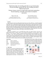
Based on a sequence of the desired footprint and
the period time of each step of the biped robot, a
reference trajectory of the ZMP can be specified.
Fig. 3 illustrates the footprint and the zigzag
reference trajectory of the ZMP to guarantee a
stable gait.

Left foot
Right foot
ZMP reference
trajectory
y [m]
x [m]

0.1
0
0.2 0.3
0.4 0.5 0.6
0.1
-0.1
t
1

t
2

t
3

t
4

t
5
t
6
t
7

t
8


Fig. 3. Footprint and reference trajectory of the

ZMP.

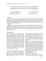
The x and y ZMP trajectories versus times
corresponding to the zigzag reference trajectory of
the ZMP in Fig. 3 can be obtained as shown in
Figs. 4 and 5.

0 10 20 30 40 50 60 70 80
-0.1
0
0.1
0.2
0.3
0.4
0.5
0.6
0.7
Time (sec)
x zmp reference
t
2

t
3

t
4

t
5

t
6

t
7

x ZMP reference input [m]


Fig. 4. x ZMP reference trajectory versus time.
Foo
0

z
c

x
a

z
a

Mass
point

x
c
a

x
zmp

Foo
0

z
c

y
a

z
a

Mass
point

y
c
a

y
zmp

Tuyển tập công trình Hội nghị Cơ điện tử toàn quốc lần thứ 6 173


Mã bài: 39

0 10 20 30 40 50 60 70 80
-0.1
-0.08
-0.06
-0.04
-0.02
0
0.02
0.04
0.06
0.08
0.1
Time (sec)
y zmp reference
t
1

t
2

t
3
t
4

t
5
t
6
t

7

t
8

y
ZMP reference input [m]


Fig. 5. y ZMP reference trajectory versus time.

3.1. Walking pattern generation based on
optimal tracking control of the ZMP
When the biped robot is modeled as the 3D
inverted pendulum which is moved on the
horizontal plane, the ZMP’s position of the biped
robot is expressed by linear independent equations
along x
a
and y
a
directions which are shown as Eqs.
(30)~(31).
cacax
xx
dt
d
u

 and

cacay
yy
dt
d
u

 are
defined as the time derivatives of the horizontal
acceleration along x
a
and y
a
directions of the
COM,
x
u and
y
u are introduced as inputs. Eqs.
(30)~(31) can be rewritten in strictly proper form
as follows:
 

 


 

,
x
x

x
g
z
01x
,u
1
0
0
x
x
x
000
100
010
x
x
x
t
ca
ca
ca
cd
zmp
x
t
ca
ca
ca
t
ca

ca
ca
x
xx
x
C
Bx
A
x































































  







   

 
.
y
y
y
g
z
01y
,u
1

0
0
y
y
y
000
100
010
y
y
y
t
ca
ca
ca
cd
zmp
y
t
ca
ca
ca
t
ca
ca
ca
y
yy




  








x
C
B
xAx






























































where
zmp
x is position of the ZMP along x
a
axis as
output of the system (32),
zmp
y is position of the
ZMP along y
a
axis as output of the system (33),
ca
x and
ca
y are positions of the COM with respect
to x

a
and y
a
axes, and
ca
x

,
ca
x


,
ca
y

,
ca
y


are
horizontal velocities and accelerations with respect
to
a
x and
a
y directions, respectively.
The systems (32) and (33) can be generalized
as a linear time invariant system as follows:

Cx
B
Ax
x



y
u

(34)
where x  
n1
is state vector of system, u
c
  is
input signal, y   is output, A  
nn
, B  
n1

and C  
1n
.
Instead of solving differential Eqs. (30)~(31),
the position of the COM can be obtained by
constructing a controller to track the ZMP as the
outputs of Eqs. (32)~(33). When
zmp

x and
zmp
y
are controlled to track the x and y ZMP reference
trajectories, the COM trajectories can be obtained
from state variables
ca
x and
ca
y . According to this
pattern, the walking or running of the biped robot
are stable.

3.2. Continuous Time Controller Design for
ZMP Tracking Control

The system (34) is assumed to be controllable and
observable. The objective designing this controller
is to stabilize the closed loop system and to track
the output of the system to the reference input.
An error signal between the reference input r(t)
and the output of the system is defined as follows:







tytrte  (35)

The objective of the control system is to regulate
the error signal e(t) equal to zero when time goes
to infinity.
As shown in Figs. 4 and 5, the x and y ZMP
reference trajectories include segments as a ramp
function and segments as a step function and have
singular points. To control the output of the ZMP
tracking control systems to track the ramp
segments of the x and y ZMP reference
trajectories, the designed controller should satisfy
the internal model principle. This means that the
reference input should be assumed to be a ramp
signal input. However, when the outputs of the
ZMP tracking control systems track the ZMP
(32)
(33)
174 Tran Dinh Huy, Nguyen Thanh Phuong, Ho Dac Loc, Tran Quang Thuan


VCM2012
reference trajectories, an overshoot occurs at
singular points of the ZMP reference input because
at these points the time derivative of the ZMP
reference input does not exist. Moreover, the
singular points of the ZMP reference trajectories
are very important points. The overshoot at these
points makes the ZMP of the biped robot to move
outside the stable region if the maximum value of
the overshoot is larger than the chosen value of
stability margin. In this case, the biped robot

becomes unstable. When the outputs of the ZMP
tracking control systems are controlled to track the
step reference inputs, the errors between the
outputs of the ZMP systems and the ramp
segments of the ZMP reference inputs are
constant. Because the ramp segments of the ZMP
reference trajectories are segments that the biped
robot changes its ZMP in two leg supported phase,
the errors mean that the outputs of the ZMP
systems are delayed by time compared with the
ZMP reference trajectories. However, the walking
pattern generation is generated in offline process
so that the errors at the ramp segments of the ZMP
reference trajectory are not important. The
reference signal is assumed to be a step function in
this paper.
The first order and second order derivatives of the
error signal are expressed as follows:







xC





 tytrte (36)
From the time derivative of the first row of Eq.
(34) and Eq. (36) the augmented system is
obtained as follows:



w
0e0edt
d
1n
aa
a
BX
X
Bx
C
0Ax

































(37)
where
uw


is defined as a new input signal.
A scalar cost function of the quadratic form is
chosen as

 




0
2
cc
dtwRJ
ac
T
a
XQX
(38)
where
   
1n1n
ecn1
1nnn
Q











0

00
Q
c
is
symmetric semi-positive definite matrix, R
c
 
and Q
ec
  are positive scalar.
The control signal w that minimizes the cost
function (38) of the system (37) can be obtained as
eKuw
c2
 xKXK
1cac


(39)
where


c
T
1cc
PBKK
1
cc2
RK


 and P
c

 
n+1n+1
is solution of the following Ricatti
equation with symmetric positive definite matrix.
0R
1
c


cc
T
aacacc
T
a
QPBBPAPPA (40)
When the initial conditions are u
c
(0) = 0 and
x(0) = 0, Eq. (39) yields

     


t
0
c2
dtteKttu xK

1c
(41)
Block diagram of the closed loop optimal
tracking control system is shown as follows:



Fig. 6. Block diagram of the closed loop optimal
tracking control system.

4. Walking Control
Based on the stable walking pattern generation
discussed in previous section, a continuous time
trajectory of the COM of the biped robot is
generated by the ZMP tracking control system.
The continuous time trajectory of the COM of the
biped robot is sampled with sampling time T
c
and
is stored into micro-controller. The ZMP reference
trajectory of the ZMP system is chosen to satisfy
the stable condition of the biped robot. The control
objective for the stable walking of the biped robot
is to track the center of the pelvis link to the COM
trajectory. The inverse kinematics of the biped
robot is solved to obtain the angle of each joint of
the biped robot. The walking control of the biped
robot is performed based on the solutions of the
inverse kinematics which is solved by the solid
geometry method.

Solving the inverse kinematics problems directly
from kinematics models is complex. An inverse
kinematics based on the solid geometry method is
presented in this section. During the walking of the
biped robot, the following assumptions are
supposed
- Trunk of the biped robot is always kept on the
sagittal plane:
42


and
69


.
- The feet of the biped robot are always parallel
with floor:
513





.
- The walking of the biped robot is divided into 3
phase: Two legs supported, right leg supported and
Tuyển tập công trình Hội nghị Cơ điện tử toàn quốc lần thứ 6 175

Mã bài: 39
left leg supported.
- The origin of the 3D inverted pendulum is
located at the ankle of supported leg.
4.2 Inverse kinematics of biped robot in one leg
supported
When the biped robot is supported by right leg,
left leg swings. A coordinate system

a
that takes
the origin at the ankle of supported leg is defined.
Since the trunk of robot is always kept on the
sagittal plane, the pelvis link is always on the
horizontal plane as shown in Fig. 7.
The knee joint angle of the biped robot is gotten as
follows:
 














21
22
2
2
1
1
3
ll2
khll
cosk

(42)
The ankle joint angle


k
2

can be obtained from
Eq. (43). The angle


k
1

can be obtained from Eq.
(44).











kh/2/lkysinAOBk
3ca
1
2



(43)
 


 


 





















1
2
2
2
1
2
1ca1
11
lkh2
llkh
cos
kh
kx
sinDOBk

(44)
where

     
kylkr
4
l
kh
ca3
2
2
3




Fig. 7 Inverted pendulum and supported leg.
4.1 Inverse kinematics of swing leg
When the biped robot is supported by right leg,
left leg is swung as shown in Fig. 8.

Fig. 8 Swing leg of biped robot.
A coordinate system
h

with the origin that is
taken at the middle of pelvis link is defined.
During the swing of this leg, the coordinate
eh
y of
the foot of swing leg is constant.



k'r
is defined
as the distance between foot and hip joint of swing
leg at k
th
sample time. It is expressed in the
coordinate system
h

as follows.
       
kz
2
l
kykxk'r
2
eh
2
3
eh
2
eh
2









(45)
where (x
eh
(k),y
eh
(k),z
eh
(k)) is coordinate of the
ankle of swing leg in the coordinate
h

at k
th
sample time.
The hip angle


k
6

of the swing leg is obtained
based on the right triangle KEF as
 


 












k'r
2/lky
sinEKFk
3eh
1
6

(46)
The minus sign in (46) means counterclockwise.
The hip angle


k
7

is equal to the angle between
link l
2
and KG line. It is can be expressed as


 

 
 
 





















2
2
1
2
2
2

1
eh
1
17
lk'r2
llk'r
cos
k'r
kx
sin
EKKGKEk

(47)
Using the cosin’s law, the angle of knee of swing
leg can be obtained as
 













21

22
2
2
1
1
18
ll2
k'rll
cosEKKk

. (48)
When robot is supported by two legs, the inverse
kinematics is calculated by similar proceduce of
one leg supported.
5. Simulation And Experimental Results
The walking control method proposed in previous
section is implemented in the CIMEC-1 biped
robot developed for this paper as shown in Fig. 9.
l
3
/2
COM
r


r


P

x
a
y
a
z
a
z
c

3

0

C

B

l
1
l
2
h



D


2

A


1

B
1
F
E
G
H
K

y
h
x
h
z
h
C

l
1

l
2
r'

(
x

ca
,
y
ca
,
z
ca
)


6


8


7

l
3
/2
K
1

176 Tran Dinh Huy, Nguyen Thanh Phuong, Ho Dac Loc, Tran Quang Thuan


VCM2012

Fig. 9. HUTECH-1 biped robot.

A simple hardware configuration using three
PIC18F4431 and one dsPIC30F6014 for the
CIMEC-1 biped robot is shown in Fig. 10.

Master unit dsPIC 30F6014

I2C communication

Motor
Motor
Motor
Potentiomate
r

Potentiomate
r

Potentiomate
r

Motor Motor
Potentiomate
r

Potentiomate
r

Motor
Motor Potentiomate
r

Potentiomate
r

Motor
Motor Potentiomate
r

Potentiomate
r

Motor
Potentiomate
r

Slave
unit
1
PIC
18
F4
431

Slave
unit
2
PIC
18
F4
431

Slave
unit
3
PIC
18
F4
431

Hip joint

Ankle joint
Hip joint

Ankle joint
Hip joint

Ankle joint
Knee joint
Hip joint

Ankle joint
Knee joint
Servo controller of right knee joint

3

Servo controller of right hip joint

5

Servo controller of right ankle joint

1

Servo controller of right hip joint

4
Servo controller of left hip joint

6

Servo controller of right ankle joint

2
Servo controller of left ankle joint

9

Servo controller of left hip joint

7

Servo controller of left ankle joint

10

Servo controller of left knee joint

8

Fig. 10. Hardware configuration of the
CIMEC-1 biped robot.

dsPIC30F6014 is used as a master unit, and
PIC18F4431 is used as slave units. The master unit
and the slave units communicate each other via
I2C communication. The master unit is used to
solve the inverse kinematics problem based on the
trajectory of the center of the pelvis of the biped
robot and the trajectory of the ankle of the
swinging leg which are contained in its memory. It
can also communicate personal computer via RS-
232 communication. The angles at the k
th
sample
time obtained from the inverse kinematics are sent
to the slave units as reference signals.
The block diagram of proposed controller for
biped robot is shown in Fig. 11.

Fig. 11 Block diagram of proposed controller.
To demonstrate the walking performance of the
biped robot based on the ZMP walking pattern
generation combined with the inverse kinematics,
the simulation results for walking on the flat floor
of the biped robot using Matlab are shown. Fig.
10. shows one step walking pattern of the biped
robot on the flat floor.

The period of step is 10 sec. That is, changing time
of supported leg is 5 sec and moving time of swing
leg is 5 sec. The length of step is 20 cm. During
the moving of the biped robot, the height of the
center of pelvis link is constant. In the swing
phase, the ZMP is located at the center of the
supported foot. When two legs of the biped robot
are contacted to the ground, the ZMP moves from
current supported leg to geometry center of the
new supported foot. The parameter values of the
biped robot used in the simulation are given in
Table 5.1.
Table 5.1 Numerical values used in simulation
Parameters Values Units
1
l

0.28 [m]
2
l

0.28 [m]
3
l

0.2

[m]
a

0.18 [m]
b

0.24

[m]
c
z

0.5 [m]

The footprint and ZMP desired trajectory are
shown in Fig. 13.
Desired
ZMP
Trajectory

x ZMP
Trajectory

y ZMP
Trajectory

y ZMP servo
system

x ZMP servo

system

x COM
y COM
Desired
trajectory of
swing leg

Biped
robot
angle joints

i

Inverse
kinematics
of the
biped
robot

Swing phase

Changing supported leg

Fig. 12 One step walking pattern.
ZMP servo system
Tuyển tập công trình Hội nghị Cơ điện tử toàn quốc lần thứ 6 177


Mã bài: 39

ZMP desired trajectory
Left foot
Right foot

Fig. 13 Footprint and desired trajectory of ZMP.
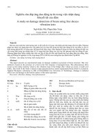
The simulation results are shown in Figs. 14~20.
Fig. 14 presents x, y ZMP reference, output and
coordinate of COM with respect to time. Figs.
15~16 show control signals and tracking errors.
Figs. 17 ~19 show joints’ angle of one leg of the
robot, the joints’ angle of opposite side leg are
similar. Fig. 20 presents movement of the center of
pelvis link in the world coordinate system.
0 10 20 30 40 50 60 70 80
-0.1
0
0.1
0.2
0.3
0.4
0.5
0.6
0.7
ZMP reference input,ZMP output, Position of COM [m]
Time [sec]
ZMP reference input
Position of COM
ZMP output

a) x ZMP reference, output and COM

0 10 20 30 40 50 60 70 80
-0.1
-0.05
0
0.05
0.1
0.15
ZMP reference input,ZMP output, Position of COM [m]
Time [sec]
ZMP reference input
Position of COM
ZMP output

a) y ZMP reference, output and COM
Fig. 14 x, y ZMP reference, output and COM.
0 10 20 30 40 50 60 70 80
-2
-1.5
-1
-0.5
0
0.5
1
1.5
2
x 10
-4
Time (sec)

Control signal u

a) Control signal u of y ZMP
0 10 20 30 40 50 60 70 80
-5
-4
-3
-2
-1
0
1
2
3
4
5
x 10
-4
Time (sec)
Control signal ux

b) Control signal u of x ZMP
Fig. 15 Control signal input.
0 10 20 30 40 50 60 70 80
-2
0
2
4
6
8
10

x 10
-3
Tracking error [m]
Time [sec]

a) x tracking error.
0 20 40 60 80
-0.025
-0.02
-0.015
-0.01
-0.005
0
0.005
0.01
0.015
0.02
0.025
Tracking error [m]
Time [sec]

b) y tracking error.
Fig. 16 Tracking error.
0 10 20 30 40 50 60 70 80
10
15
20
25
30
35

40
45
50
55
Time (sec)
Ankle joint angle 
1
(deg)
Experiment Result
Simulation result

Fig. 17 The ankle joint angle
1

.
0 10 20 30 40 50 60 70 80
-15
-10
-5
0
5
10
15
20
Time (sec)
Ankle joint angle 
2
(deg)
Experiment result
Simulation result

Fig. 18 The ankle joint angle
2

.
0 10 20 30 40 50 60 70 80
40
45
50
55
60
65
70
75
80
85
90
95
Time (sec)
Knee joint angle 
3
(deg)
Experiment result
Simulation result

Fig. 19 The knee joint angle
3

.
[m]

[m]

[m]

[m]

178 Tran Dinh Huy, Nguyen Thanh Phuong, Ho Dac Loc, Tran Quang Thuan


VCM2012
-0.1 0 0.1 0.2 0.3 0.4 0.5 0.6 0.7
-0.1
-0.05
0
0.05
0.1
x (m)
y (m)

Fig. 20 Coordinate of center of pelvis link.
5. Conclusion
In this paper, a 10 DOF biped robot is developed.
The kinematic and dynamic models of the biped
robot are proposed. An continuous time optimal
tracking controller is designed to generate the
trajectory of the COM for its stable walking. The
walking control of the biped robot is performed
based on the solutions of the inverse kinematics
which is solved by the solid geometry method. A

simple hardware configuration is constructed to
control the biped robot. The simulation and
experimental results are shown to prove
effectiveness of the proposed controller.
REFERENCES
[1] S. Kajita, F. Kanehiro, K. Kaneko, K, Yokoi
and H. Hirukawa, “The 3D Linear Inverted
Pendulum Mode: A simple modeling for a
biped walking pattern generation”, Proc. of
IEEE/RSJ International conference on
Intelligent Robots and Systems, pp. 239~246,
2001.
[2] C. Zhu and A. Kawamara, “Walking Principle
Analysis for Biped Robot with ZMP Concept,
Friction Constraint, and Inverted Pendulum
Model”, Proc. of IEEE/RSJ International
conference on Intelligent Robots and Systems,
pp. 364~369, 2003.
[3] S. K. Agrawal, and A. Fattah, “Motion
Control of a Novel Planar Biped with Nearly
Linear Dynamics”, IEEE/ASME Transaction
on Mechatronics, Vol. 11, No. 2, pp.
162~168, 2006.
[4] J. H. Part, “Impedance Control for Biped
Robot Locomotion”, IEEE Transaction on
Robotics and Automation, Vol. 17, No. 3, pp.
870~882, 2001.
[5] Q. Huang and Y. Nakamura, “Sensor Reflex
Control for Humanoid Walking”, IEEE
Transaction on Robotics, Vol. 21, No. 5, pp.

977~984, 2005.
[6] B. C. Kou, “Digital Control Systems”,
International Edition, 1992.
[7] D. Li, D. Zhou, Z. Hu, and H. Hu, “Optimal
Priview Control Applied to Terrain Following
Flight”, Proc. of IEEE Conference on
Decision and Control, pp. 211~216, 2001.
[8] D. Plestan, J. W. Grizzle, E. R. Westervelt and
G. Abba, “Stable Walking of A 7-DOF Biped
Robot”, IEEE Transaction on Robotics and
Automation, Vol. 19, No. 4, pp. 653-668,
2003.
[9] F. L. Lewis, C. T. Abdallah and D.M.
Dawson, “Control of Robot Manipulator”,
Prentice Hall International Edition, 1993.
[10] G. F. Franklin, J. D. Powell and A. E. Naeini,
“Feedback Control of Dynamic System”,
Prentice Hall Upper Saddle River, New Jersey
07458.
[11] G. A. Bekey, “Autonomous Robots From
Biological Inspiration to Implementation and
Control”, The MIT Press 2005.
[12] H. K. Lum, M. Zribi and Y. C. Soh, “Planning
and Control of a Biped Robot”, International
Journal of Engineering Science ELSEVIER,
Vol. 37, pp. 1319~1349, 1999.
[13] H. Hirukawa, S. Kajita, F. Kanehiro, K.
Kaneko and T. Isozumi, “The Human-size
Humanoid Robot That Can Walk, Lie Down
and Get Up”, International Journal of

Robotics Research Vol. 24, No. 9, pp.
755~769, 2005.
[14] K. Mitobe, G. Capi and Y. Nasu, “A New
Control Method for Walking Robots Based on
Angular Momentum”, Journal of
Mechatronics ELSEVIER, Vol. 14, pp.
164~165, 2004.
[15] K. Harada, S. Kajita, K. Kaneko and H.
Hirukawa, “Walking Motion for Pushing
Manipulation by a Humanoid Robot”, Journal
of the Robotics Society of Japan, Vol. 22, No.
3, pp. 392–399, 2004.

Tran Dinh Huy received the B.E. and
M.E. degrees in mechanical
engineering from HoChiMinh City
University of Technology in 1995 and
1998, respectively. He is currently a
PhD. student of Open University
Malaysia. His research interests include robotics
and motion control.

Nguyen Thanh Phuong received
the B.E., M.E. degrees in electrical
engineering from HoChiMinh City
University of Technology, in 1998,
2003, and PhD degree in
mechatronics in 2008 from Pukyong
National University, Korea respectively. He is
currently a Lecturer in the Department of

Tuyển tập công trình Hội nghị Cơ điện tử toàn quốc lần thứ 6 179


Mã bài: 39
Mechanical – Electrical - Electronic,HUTECH
university. His research interests include robotics,
renewable energy and motion control.

Ho Dac Loc received the B.E., PhD.
and Dr.Sc. degrees in electrical
engineering from Russia, in 1991,
1994 and 2002, respectively. He is
currently a rector of HUTECH
university. His research interests include robotics
and industrial automatic control.

Tran Quang Thuan received the
B.E. and M.E. degrees in electrical -
electronic engineering from
HoChiMinh City University of
Technology in 1998 and 2006,
respectively. He is currently a
Lecturer, of Faculty of Electronics Engineering,
Posts and Telecommunications Institute of
Technology branch Hochiminh city and a PhD.
student of Vietnam Research Institute of
Electronics, Informetics and Automation. His
research interests include robotics and motion
control.