Proceedings VCM 2012 25 discrete time optimal tracking control of BLDC motor
Bạn đang xem bản rút gọn của tài liệu. Xem và tải ngay bản đầy đủ của tài liệu tại đây (469.53 KB, 7 trang )
180 Tran Dinh Huy, Nguyen Thanh Phuong, Vo Hoang Duy and Nguyen Van Hieu
VCM2012
Discrete Time Optimal Tracking Control of BLDC Motor
Tran Dinh Huy, Nguyen Thanh Phuong, *Vo Hoang Duy and **Nguyen Van Hieu.
Ho Chi Minh City University of Technology, Vietnam
* Ton Duc Thang University
** A41 Manufactory, Ministry of Defence
e-Mail:
Abstract:
Brushless Direct Current (BLDC) motors are widely used for high performance control applications.
Conventional PID controller only provides satisfactory performance for set-point regulation. In this paper, a
discrete time optimal tracking control of BLDC motor is presented. Modeling of the BLDC motor is expressed
in state equation. A discrete time full-order state observer is designed to observe states of BLDC motor.
Feedback gain matrix of the observer is obtained by pole assignment method using Ackermann formulation
with observability matrix. The state feedback variables are given by the state observer. A discrete time LQ
optimal tracking control of the BLDC motor system is constructed to track the angle of rotor of the BLDC
motor to the reference angle based on the designed observer. Numerical and experimental results are shown to
prove that the performance of the proposed controller.
1. Introduction
The disadvantages of DC motors emerge due to
the employment of mechanical commutation since
the life expectancy of the brush construction is
restricted. Furthermore, mechanical commutators
lead to losses and contact uncertainties at small
voltages and can cause electrical disturbances
(sparking). Therefore, Brushless Direct Current
(BLDC) motors have been developed. BLDC
motors do not use brushes for commutation;
instead, they are electronically commutated.
BLDC motors are a type of synchronous motor.
This means that the magnetic field is generated by
the stator and the rotor which rotates at the same
frequency so that the BLDC motor do not
experience the “slip” that is normally seen in
induction motors. In addition, BLDC motor has
better heat dissipation characteristic and ability to
operate at higher speed [1]. However, the BLDC
motor constitutes a more difficult problem in terms
of modeling and control system design due to its
multi-input nature and coupled nonlinear
dynamics.
Therefore, a compact representation of the BLDC
motor model was obtained in [2]. This model is
similar to permanent magnet DC motors. As a
result, PID controller can be easily applied to
control BLDC motors. In recent years, researchers
had applied another algorithm to enhance high
performance system. R. Singh presented DC motor
predictive models [5], this research designed
optimal controller also. M. George introduced
speed control of separated excited DC motor [4].
GUPTA presented a robust variable structure
position control of DC motor [6]. These researches
focused in continuous time system so that
implementation of microcontroller is not
convenient.
This paper presents a discrete time optimal
tracking control of BLDC motor. The model of the
BLDC motor is expressed as discrete time
equations. The optimal tracking controller based
on the estimated states by using discrete time
observer is designed to control. The effectiveness
of the designed controller is shown via numerical
and experimental results in the comparing with the
traditional PID controller.
2. Brushless DC Motors
Unlike a permanent magnet DC motor, the
commutation of a BLDC motor is controlled
electronically. To rotate the BLDC motor, the
stator windings should be energized in a sequence.
It is important to know the rotor position in order
to understand which winding will be energized
following the energizing sequence. Rotor position
is sensed using Hall effect sensors embedded into
the stator.
The dynamic characteristics of BLDC motors are
similar to brushed DC motors. The model of
BLDC motor can be represented as [2].
Tuyển tập công trình Hội nghị Cơ điện tử toàn quốc lần thứ 6 181
Mã bài: 40
iKT
tm
(1)
e
KE
(2)
KiTbJ
m
(3)
KVRi
dt
di
L
(4)
where
R : Armature resistance [].
L : Armature inductance [H].
K : Electromotive force constant [Nm/A].
K
t
: Torque constant [Nm/A].
K
e
: Voltage constant [Vs/rad].
V : Source voltage [V].
: Angular velocity of rotor [rad/s].
J : Moment of inertia of the rotor [kgm
2
].
b : Damping ratio of the mechanical system
[Nms].
In SI unit system, Kt is equal to Ke.
Combining (3) and (4) yields
KVKRbRJLbLJ
2
(5)
T
m
x is defined as state vector of the
BLDC motor. Eq. (5) can be written as
m
m
m
m
m
m
x
C
B
x
A
x
001
0
0
0
100
010
2
m
y
V
LJ
K
LJ
RJLb
LJ
KRb
(6)
where
m
y is rotational angle of the rotor of the
BLDC motor.
The discrete time system equations of the BLDC
motor can be obtained as
kTky
kVTkTk
m mm
mmmm
xC
θxΦx
1
(7)
where
13
k
m
x is state vector of the BLDC motor at
the k
th
sample time,
ky
m
is rotational angle of the rotor of the
BLDC motor at the k
th
sample time,
3332
!
3
1
!
2
1
TTTeT
T 32
m3
A
m
mm
m
AAAIΦ
,
13
0
dTT
T
BΦθ
mm
, and
31
mm
CC T
3. CONTROLLER DESIGN
3.1 Discrete Time Full-Order State Observer
Design
To implement the discrete time optimal tracking
controller, the information of all state variables of
the system is needed. However, all state variables
are not accessible in practical systems [3].
Furthermore, in the system that all state variables
are accessible, the hardware configuration of the
system becomes complex and the cost to
implement this system is very high because
sensors to measure all states are needed. Because
of these reasons, a discrete time observer is needed
to estimate the information of all states of the
system. In the case that the output of the system is
measurable and the system is full-observable, a
discrete time full-order state observer can be
designed to observe information of all state
variables of the system.
It is assumed that the system (7) is full-observable.
The system equations of the discrete time closed
loop observer are proposed as follows:
kTky
kykykVTkTk
m
mm
mm
mmmm
xC
LθxΦx
ˆ
ˆ
ˆ
ˆ
1
ˆ
(8)
where
13
ˆ
k
m
x
is state vector of the observer at
the k
th
sample time,
ky
m
ˆ
is the rotational
angle of rotor of the observer at the k
th
sample
time, and
13
L
is the feedback gain matrix.
kkk
mmm
xxx
ˆ
~
is defined as the estimated
error state vector between the motor and the
observer. Subtracting Eq. (8) from Eq. (7), the
error state equation can be obtained as
kkTTk
mcdmmmm
xAxLCΦx
~
~
1
~
(9)
The design objective of the observer is to obtain a
feedback gain matrix
L
such that the estimated
error states approach to zero as fast as possible.
That is, the feedback gain matrix
L
must be
designed such that eigenvalues of A
cd
exist in unit
circle for the system (9) to be stable. By pole
assignment method using Ackermann formulation
with observability matrix O
m
, the feedback gain
matrix
L
is obtained as follows [3]:
1
0
0
''
1
2
mm
mm
m
m
T
3
1
mm
ΦC
ΦC
C
ΦeOΦL
(10)
where
m
Φ' is desired characteristic equation of
the observer,
T
2
mmmmmm
ΦCΦCCO
is
observability matrix, and
100
3
e is unit
vector.
Block diagram of this observer is shown in Fig. 1.
182 Tran Dinh Huy, Nguyen Thanh Phuong, Vo Hoang Duy and Nguyen Van Hieu
VCM2012
Figure 1 Block diagram of the system with
observer.
3.2 Discrete time optimal controller design
based on discrete time full-order state
observer
The discrete time state variables equation of the
BLDC motor can be rewritten as follows:
kk
kkk
xCy
uBxAx
d
dd
1
(11)
where x(k)
31
is state vector, y(k) is
output, u(k)
is control input, and A
d
33
,
B
d
31
, C
d
13
are matrices with
corresponding dimensions.
An error signal e(k) is defined as the
difference between the reference input r(k)
and the output of the system y(k) as follows:
kkk yre (12)
It is denoted that the incremental control input
is
1 kkk uuu and the incremental state is
1 kkk xxx . If the system (11) is
controllable and observable, it can be rewritten in
the increment as follows:
kk
kkk
xCy
uBxAx
d
dd
1
(13)
The error at the k+1
th
sample time can be obtained
from Eq. (12) as
111 kkk yre . (14)
Subtracting Eq. (12) from Eq. (14) yields
kkkkkk yyrree 111
(15)
Substituting Eq. (13) into Eq. (15) can be reduced
as
kkkkk uBCxACree
dddd
11
(16)
where
kkk rrr 11
It is assumed that future values of the reference
input
,,2,1
kk rr cannot be utilized. The
future values of the reference input beyond the k
th
sample time are approximated as
kr . It means
that the following is satisfied.
,2,1for0 iikr (17)
From the first row of Eq. (13) and Eq. (16), the
error system can be obtained as
k
k
k
k
k
kk
u
B
BC
x
e
A0
AC1
x
e
G
d
dd
X
A
d3x1
dd
X
E
1
1
1
(18)
where
14
kX
,
44
E
A
, and
14
G .
A scalar cost function of the quadratic form is
chosen as
0k
kΔkΔkkJ uRuXQX
TT
(19)
where
44
3
313
31e
00
0Q
Q
is semi-positive
definite matrix,
e
Q , and
R
are positive
scalar.
The optimal control signal
ku that minimizes
the cost function (19) of the system (18) can be
obtained as [3]
kk XAPGGPGRu
E1
T
1
1
T
(20)
where
P
is semi-positive definite matrix. It is
solution of the following algebraic Ricatti equation
[3].
E
T
1
TT
EE
T
E
PAGPGGPGAPAAQP
R
(21)
where
44
Q
is semi-positive definite matrix,
and
R
is positive scalar.
By taking the initial values as zero and integrating
both side of Eq. (20), the control law
ku can be
obtained as
kke
z
z
Kku
e m1x
xK
1
1
(22)
where
41
E1
T
1
1
T
1x1e1
APGGPGRKK K
Based on the proposed observer (9) and the
controller (22), the discrete time optimal controller
design based on discrete time full-order state
observer can be given as follows:
kke
z
z
KkV
e m1x
xK
ˆ
1
1
(23)
The discrete time optimal tracking control system
of the BLDC motor (7) designed based on the
information of states of the system obtained from
Tuyển tập công trình Hội nghị Cơ điện tử toàn quốc lần thứ 6 183
Mã bài: 40
discrete time closed loop observer (9) is shown in
Fig. 2.
Figure 2 Block diagram of the optimal control of
the BLDC motor.
4. Numerical And Experimental Results
The specification of BLDC motor is shown in
Table 1.
The effectiveness of the controller (23) as shown
in Fig. 2 is verified by the simulation and
experimental results.
The BLDC motor is controlled by the optimal
tracking controller (23) which is obtained by
choosing
1
R
and
0000
0000
0000
0002.0
Q . The poles
of the system (9) are chosen as
j0.32 - 0.375j0.32 + 0.3755.0λ for fast
response. The feedback gain matrix
T
00000012.000009.0153.0L is obtained
from (10). The simulation results of the observer
are shown in Figs. 3~5. And the simulation results
of the designed discrete time optimal tracking
controller of BLDC motor designed based on the
discrete time full-order state observer are shown in
Figs. 6~9.
Figs. 3~6 show that even with different initial
conditions between observer and system, all states
and the output of the designed observer converge
to those of system after about 0.01 second.
Fig. 7 shows that discrete time optimal tracking
controller of the BLDC motor designed based on
the discrete time full-order state observer has good
performance. The output of the system converges
to the reference input after about 0.08 second, and
its overshoot is about 4.5%. The tracking error of
the system is shown in Fig. 8. The control signal
input is shown in Fig. 9.
Figs. 10~15 show the simulation results of the
tracking angle of the BLDC motor control system
using the PID controller with two cases:
unbounded control signal and bounded control
signal. The proposed PID controller is designed
based on the flat criterion. When control signal V
is unbounded, the overshoot of the output is about
11.5% as shown in Fig. 10, and tracking error
converges to zero after about 0.07 second as
shown in Fig. 11. However, the control signal V
changes from -2000 to 4100 as shown in Fig. 12, it
is too big value to be implemented for the real
system. When the control signal V is bounded as
shown in Fig. 15, overshoot of the output is about
40% as shown in Fig. 13, and tracking error
converges to zero after about 0.08 second as
shown in Fig. 14.
In comparing the simulation results of the
designed discrete time optimal tracking controller
designed based on discrete time full-order state
observer with those of the proposed PID
controller, it is shown that the designed discrete
time optimal tracking controller has better
performance than the proposed PID controller.
Table 1 Specification of BLDC motor
Parameters Values and units
R 21.2 Ω
K
e
0.1433 V s/rad
D 1x10
-4
kg-m s/rad
L 0.052H
K
t
0.1433 kg-m/A
J 1x10
-5
kg-m s
2
/rad
0 0.02 0.04 0.06 0.08 0.1
0
2
4
6
8
10
12
Time [sec]
State x
1
of plant and observer [deg]
State of plant
State of observer
Figure 3 State θ
ˆ
of observer and state
θ
of
plant.
ˆ
184 Tran Dinh Huy, Nguyen Thanh Phuong, Vo Hoang Duy and Nguyen Van Hieu
VCM2012
0 0.02 0.04 0.06 0.08 0.1
-50
0
50
100
150
200
250
300
350
400
Time [sec]
State x
2
of plant and observer [rad/s]
State of plant
State of observer
Figure 4 State
θ
ˆ
of observer and state θ
of plant.
0 0.02 0.04 0.06 0.08 0.1
-4
-3.5
-3
-2.5
-2
-1.5
-1
-0.5
0
0.5
1
x 10
5
Time [sec]
State x
3
of plant and observer
State of plant
State of observer
Figure 5 State
θ
ˆ
of observer and state θ
of
plant.
0 0.005 0.01 0.015 0.02
-1
-0.8
-0.6
-0.4
-0.2
0
0.2
0.4
Time [sec]
Error between output of observer and plant [deg]
Figure 6 Error between estimated output of
observer and output of plant.
0 0.05 0.1 0.15
0
1
2
3
4
5
6
7
8
9
10
11
Time [sec]
Reference input and output [deg]
Output
Reference input
Figure 7 Reference input and output of system
using optimal controller.
0 0.05 0.1 0.15
-2
0
2
4
6
8
10
Time [sec]
Tracking error [deg]
Figure 8 Tracking error of system using discrete
time optimal controller.
0 0.05 0.1 0.15
-5
0
5
10
15
20
25
Time [sec]
Control signal V [V]
Figure 9 Control signal input using discrete time
optimal controller.
0 0.05 0.1 0.15
0
2
4
6
8
10
12
Time [sec]
Reference input and output of system [deg]
Reference input
Ouput of the system
Figure 10 Reference and output of system using
PID controller with unbounded control signal V.
0 0.05 0.1 0.15
-2
0
2
4
6
8
10
Time (sec)
Tracking error
Figure 11 Tracking error of system using PID
controller with unbounded control signal V.
[
deg]
[rad/s
2
]
ˆ
ˆ
Tuyển tập công trình Hội nghị Cơ điện tử toàn quốc lần thứ 6 185
Mã bài: 40
0 0.05 0.1 0.15
-2000
-1000
0
1000
2000
3000
4000
5000
Time (sec)
Control signal V
Figure 12 Unbounded control signal V of PID
controller.
0 0.05 0.1 0.15
0
5
10
15
Time [sec]
Reference input and output of the system [deg]
Reference input
Ouput of the system
Figure 13 Reference and output of system using
PID controller with bounded control signal V.
0 0.05 0.1 0.15
-5
0
5
10
Time (sec)
Tracking error
Figure 14 Tracking error of system using PID
controller with bounded control signal V.
0 0.05 0.1 0.15
-500
-400
-300
-200
-100
0
100
200
300
400
500
Time (sec)
Control signal input V
Figure 15 Bounded control signal V of PID
controller.
To illustrate the effectiveness, a position tracking
control scheme of BLDC motor is implemented.
The experimental set up is shown in Fig. 16. A
BLDC motor driver is built using Hex MOSFET
IRF540, IR2101 as a gate driver, and encoder as a
speed feedback sensor. The main controller is
PIC18F4431 Microchip. Fig. 17 shows each phase
hall sensor signals versus phase voltages in Fig.
18.
Figure 16 Developed speed control of BLDC
motor system
Voltage (V)
Time (ms)
0 2.5 5 7.5 10 12.5 15 17.5 20 22.5 25
0
10
0
10
0
Figure 17 Hall sensor signals
Voltage (V)
Time (ms)
0 2.5 5 7.5 10 12.5 15 17.5 20 22.5 25
0
50
0
50
0
Figure 18 Motor phase voltages
[
deg]
186 Tran Dinh Huy, Nguyen Thanh Phuong, Vo Hoang Duy and Nguyen Van Hieu
VCM2012
5. Conclusion
In this paper, a discrete time optimal tracking
control system for BLDC motor based on a full-
order observer has been applied and investigated
to control position of BLDC motor. Performance
of the optimal tracking controller is analyzed and
compared with the traditional PID controller. The
effectiveness of the designed controller is shown
by the simulation and experimental results.
Moreover, the responses of the system using
discrete time optimal and proposed PID controller
are presented to compare their performance.
References
[1] N. Hemati, “The global and local dynamics of
direct-drive brushless DC motors”, In
proceedings of the IEEE power electronics
specialists conference, (1992), pp. 989-992.
[2] Chee-Mun Ong, “Dynamic simulation of
electric machinery”, Prentice Hall, (1998).
[3] B. C. Kou, “Digital Control Systems”,
International Edition, 1992.
[4] M. George “Speed Control of Separated
Excited DC Motor”, American journal of
applied sciences, Vol. 5, 227~ 233, 2008.
[5] R. Singh, C. Onwubolu, K. Singh and R. Ram,
“DC Motor Predictive Model”, American
journal of applied sciences, Vol. 3, 2096~ 2102,
2006.
[6] M. K. Gupta, A. K Shama and D. Patidar, “A
Robust Variable Structure Position Control of
DC Motor”, Journal of theoretical and applied
information technology, 900~905, 2008.
Tran Dinh Huy received the B.E.
and M.E. degrees in mechanical
engineering from HoChiMinh City
University of Technology in 1995 and
1998, respectively. He is currently a
PhD. student of Open University Malaysia. His
research interests include robotics and motion
control.
Nguyen Thanh Phuong received the
B.E., M.E. degrees in electrical
engineering from HoChiMinh City
University of Technology, in 1998,
2003, and PhD degree in
mechatronics in 2008 from Pukyong
National University, Korea respectively. He is
currently a Lecturer in the Department of
Mechanical – Electrical - Electronic,HUTECH
university. His research interests include robotics,
renewable energy and motion control.
Vo Hoang Duy received the B.E.,
M.E. degrees in electrical engineering
from HoChiMinh City University of
Technology, in 1997, 2003, and PhD
degree in mechatronics in 2007 from
Pukyong National University, Korea respectively.
He is currently a Lecturer in the Department of
Electrical - Electronic, Ton Duc Thang university.
His research interests include robotics and
industrial automatic control.
Nguyen Van Hieu received the B.E.,
degree in Mechanical engineering from
HoChiMinh City University of
Technology, in 1993, M.E., and PhD
degrees in Automatic control
engineering in 2010 and 2012 from IASS, Russia
respectively. He is currently a Vice director of
A41 manufactory. His research interests include
robotics and automotive engineering.