Weather shocks and nutritional status of disadvantaged children in Vietnam

WP 13/10
Weather shocks and nutritional status of disadvantaged
children in Vietnam
Ijeoma P. Edoka
May 2013
york.ac.uk/res/herc/hedgwp


1

Weather shocks and nutritional status of disadvantaged children in
Vietnam


Ijeoma P. Edoka
*

Institute for International Health and Development, Queen Margaret University,
Edinburgh EH21 6UU

May, 2013




Abstract

This study uses the Vietnam Young Lives Survey to investigate the impact of small-scale weather shocks
on child nutritional status as well as the mechanism through which weather shocks affect child nutritional
status. The results show that small-scale weather shocks negatively affect child nutritional status and total
household per capita consumption and expenditure (PCCE) but not food PCCE. Disaggregating total

food PCCE into consumption of high-nutrient and energy-rich food shows that households protect food
consumption by decreasing consumption of high-nutrient food and increasing consumption of affordable
but low quality food. This suggests that the impact of small-scale weather shocks on child health is
mediated through a reduction in the quality of dietary intake. Finally, this study shows evidence of a
differential impact of weather shocks in children from different socioeconomic backgrounds. The impact
of weather shocks is observed to be greater amongst children from wealthier households compared to
children from poorer households.

JEL classification: I1, O1
Keywords: Weather shocks, Height-for-age Z-scores, Household consumption



*
Email:


2

1 Introduction

The increasing frequency of occurrence and the devastating impact of weather shocks represent
a growing concern globally, particularly in developing countries where the impact is further
exacerbated by the lack of adequate infrastructures and facilities capable of mitigating the
immediate impact or aftermaths of weather shocks (Kahn, 2005; UNISDR, 2011b). The
enormous human and welfare losses associated with weather shocks are widely documented. For
example, in 2011 alone, approximately 332 weather shocks where reported worldwide, affecting
244.7 million and killing over 30,000 with a total economic cost estimated at approximately 366.1
billion US dollars (Guha-Sapir et al., 2012). Other specific examples include the 2010 earthquake
in Haiti in which an estimated 250,000 persons were killed or missing, incurring a total damage

estimated at approximately 8.1 billion US dollars (Cavallo et al., 2010). The boxing day Indian
Ocean tsunami in 2004 caused large-scale destruction with an estimated death toll of over
165,000 in Indonesia alone and over 200,000 deaths across 12 affected countries including
Thailand, India and Sri Lanka (Cavallo et al., 2010; Keys et al., 2006). Other weather shocks such
as floods and landslides, droughts and volcanic eruptions cause similar large-scale human and
economic losses (Guha-Sapir et al., 2012). In addition to the immediate impact, weather shocks
often result in huge secondary public health crises resulting from the outbreak of diseases, the
disruption of safe drinking water supply and sanitation, the displacement of families and the
relocation of survivors into crowded rescue centres, exposing survivors to further health hazards
(Watson et al., 2007).
Children are particularly vulnerable and approximately 30-50% of fatalities resulting from the
immediate repercussions of weather shocks are reported to be children (UNISDR, 2011a).
Furthermore, weather shocks have been implicated in long-term child health outcomes including
higher morbidity and mortality amongst children long after they survive the immediate impact.
For example, following extreme drought in Zimbabwe, exposed children experienced slower
growth rates (Hoddinott & Kinsey, 2001), the 1997 forest fire in Southeast Asia resulted in
higher infant and child mortality in Indonesia (Jayachandran, 2009), while the 1998 Hurricane
Mitch affecting large parts of Central America was associated with an increase in the prevalence
of wasting and malnutrition amongst affected children in Honduras and Nicaragua (Barrios et al.,
2000).
There is a growing body of evidence showing links between child stature and future labour
market achievements (Case and Paxson (2008), and references therein). Therefore, shocks which


3

affect child physical development and growth are likely to have long-term economic
consequences. For example, Alderman et al. (2006) showed that in addition to childhood
stunting, exposure to drought and civil war in early childhood resulted in lower educational
attainment in adulthood. Other studies have equally highlighted the long-term health and

economic consequences of other forms of early childhood shock. Some examples include higher
mortality rates amongst adults born during an economic downturn compared to those born
during an economic boom (van den Berg et al., 2006); shorter height at age 20 amongst cohorts
whose parents experienced income shocks resulting from a widespread destruction of vineyards
in mid-19
th
century France (Banerjee et al., 2010); lower educational attainment and occupational
status amongst adults born during the food crisis in Germany following World war II, compared
to those born shortly before or after the crisis (Jürges, forthcoming).
Previous research on weather shocks and child health has focused mainly on the impact of single
large-scale weather shocks on child health with fewer studies on the impact of smaller-scale
weather shocks. Although the human and economic costs of smaller-scale weather shocks are
likely to be less compared to large-scale shocks, recurrent exposure to small-scale weather shocks
are likely to have significant impacts on household welfare as well as on children’s short- and
long-term health outcomes. To the best of my knowledge only two studies have investigated the
impact of small-scale weather shocks on child health. Pörtner (2010) showed using three rounds
of the Guatemala Demographic and Health Surveys (DHS), that exposure to hydro-metrological
disasters (storms, flooding, heavy rainfall, hurricanes and frost) has a negative impact on child’s
health. After controlling for area and time fixed effects, exposure to small-scale weather shocks
in the past year was associated with lower nutritional status in children under 5 years of age
(Pörtner, 2010). Similar findings were reported by Datar et al. (2011) in rural India. Using
repeated cross-sections of the National Family Health Surveys (NFHS), Datar et al. (2011)
showed that exposure to different small-scale weather shocks in the previous year reduced child
height-for-age Z-score (HAZ-score) by approximately 0.12-0.15 standard deviations and
increased the probability of reporting symptoms of acute illnesses by 9-18% (Datar et al., 2011).
HAZ-scores are regarded as a long-run indicator of child nutritional status and are estimated by
standardising child height using the median height of a well-nourished child of the same age and
gender in a reference population (where the United States National Centre for Health Statistics
(US NCHS) sample is used as the reference population). Low HAZ-scores are indicative of past
disruptions to child nutritional status resulting from inadequate food nutrient intake and/or

recurrent infections and illnesses. The HAZ-score is widely used as a proxy for child health and
is an important determinant of child’s future health outcomes. For example, childhood


4

malnutrition and wasting (HAZ-score less that -2) is associated with higher morbidity and
mortality in adulthood (Victora et al., 2008).
In addition to fatalities and injuries resulting from the direct repercussions of weather shocks,
shock to household income and changes in parental behaviour such as investment decisions in
child health represent possible mechanisms through which weather shocks affect child health. In
developing countries, the immediate and long-term impact of weather shocks on household
welfare is well documented. Significant reductions in both agricultural and non-agricultural wages
have been reported several years after the occurrence of a natural disaster (Jayachandran, 2006;
Mueller & Osgood, 2009; Mueller & Quisumbing, 2010; T. Thomas et al., 2010). Since child
health is a function of a set of inputs such as food nutrients, time and resources invested in
caring for the child (Behrman & Deolalikar, 1988; Grossman, 1972; Rosenzweig & Schultz,
1983), shocks to household income are likely to reduce the demand for these inputs, potentially
making child health vulnerable. In addition, shocks to household income may increase the
opportunity cost of parents time in caring for the child when the need to replenish lost income
and for day-to-day subsistence supersedes the need to investment in child health. For example,
Datar et al. (2011) showed that in addition to the impact on child’s nutritional status, children
exposed to small-scale weather shocks are less likely to have full age-appropriate immunization
coverage. Similar findings are reported by Miller and Urdinola (2010) who show an association
between weather-induced increases in coffee prices and a decline in the use of preventative care
and vaccination services during the first year of a child’s life. Furthermore, the need to generate
extra income may result in children having to contribute to household income and an increase in
the supply of child labour, further compromising child health outcomes (O'Donnell et al., 2002;
Roggero et al., 2007).
This study contributes to this literature by estimating the impact of small-scale weather shocks

on both child health and household income
1
. It differs from previous studies which have either
estimated the impact of weather shocks on child health or on household income, by estimating
the impact of small-scale weather shocks on both child health and on household income using
the same sample. Thus, this study is able to explicitly demonstrate that the adverse impact of
weather shocks on child health is mediated through a reduction in household income. It uses the

1
Household per capita consumption and expenditure (PCCE) on all goods including food and non-food goods
(excluding medical care expenditures) is used as a proxy for household income.




5

2006 and 2009 panels of the Vietnam Young Lives Surveys (VYLS), which consist of a pro-poor
sample of children aged 4 and 12 years in 2006.
Consistent with other studies, a negative association is observed between small-scale weather
shocks and child HAZ-scores as well as between household total (log) per capita consumption
and expenditure (PCCE). The analysis is extended to assess the impact on the quantity
(household total PCCE on food) and the quality (household PCCE on high-nutrient and energy-
rich food) of dietary intake. No statistically significant difference is observed in total food
consumption between exposed and unexposed households. However, the results suggest that
exposed households are able to smooth consumption of total food by decreasing the
consumption of high-nutrient food (fish, meat, fruits and vegetables) by approximately the same
magnitude as their increase in the consumption of low-nutrient, high calorie food (rice and
tubers). This is indicative of a fall in quality of households’ food intake, thus, providing an
explanation for the negative impact of small-scale weather shocks on child nutritional status.

Disadvantaged groups such as children living in poorer households have been shown to more
vulnerable to weather shocks (Datar et al., 2011; Hoddinott & Kinsey, 2001), therefore this study
also investigates the extent to which differential impact of small-scale weather shocks on
household PCCE explains differential impact on child HAZ-score.
The rest of the paper is organized as follows: the conceptual framework and econometric
models are outlined in sections 2 and 3, respectively. Section 4 provides a description the VYLS
and variables included in econometric models. The results are presented in section 5 and section
6 concludes by summarizing the key findings of the study.

2 Conceptual Framework

Following the literature on the demand for child health
2
, the conceptual framework adopted in
this study relies on a model of child health production in which child health is embedded in a
household utility function. Households are assumed to maximise a utility function at time t
given as:
  



 

 







2
Some examples include Pitt and Rosenzweig (1985), Thomas et al. (1990), Alderman and Garcia (1994) Hoddinott
and Kinsey (2001) and Behrman and Skoufias (2004)


6

where C is a vector of goods consumed (health and non-health goods), H is a vector of home-
produced commodities such as child health, and K is a vector of household characteristics which
may affect utility. Households face two constraints in the production of commodities: a
constraint imposed by the technology through which it combines goods to produce commodities
(technological constraint) and a budget constraint which determines the bundle of goods it can
afford. Thus, the maximization problem facing households is subject to a budget constraint,
households’ technology and a child health production function.
The child health production function can be described as a function of a set of inputs which can
be combined to produce child health. These inputs such as food nutrients, time and resources
invested in caring for the child are demanded by parents because they affect parents’ utility
indirectly through their impact on child health. In this study, child HAZ-score or nutritional
status is used as an indicator of child health. Child nutritional status is described as a function of
a set of material and environmental inputs which affect child stature:


 



 


 

 

 

 

 

 



where H is the child’s HAZ-score, X is a vector of observable child characteristics such as age
and gender which may affect growth rate, Z is household consumption and expenditure on food
nutrients which captures food nutrient input, M is a vector of non-material inputs such as time
invested in caring for the child, P is a vector of parental characteristics such as education and age
which may affect the technology through which health inputs are combined, K is a vector of
household characteristics capturing the health environment facing each child such as good
sanitation and availability of safe drinking water, 

captures time-invariant unobserved child
characteristics such as genetic predispositions which are uninfluenced by parental behaviours or
preferences but which may affect child health and 

and 

are unobserved time-invariant
household and community characteristics, respectively, which could also affect child health.

Weather shocks are often associated with economic and welfare losses, particularly in poor
households already facing huge budget constraints and limited abilities to smooth consumption.
This may in turn affect child’s nutritional status through a reduction in household food
consumption and expenditure. Household food consumption and expenditure, Z, is described as
follows:


 


 

 

 




7

where 


represents households’ exposure to small-scale weather shocks between time periods
t and t -1,  is household income (or total PCCE on all food and non-food goods) and 

are
unobserved time-invariant household and community characteristics that could affect household
food consumption and expenditure. Substituting equation (3) into (2), yields a child health

production function that includes households’ exposure to small-scale weather shocks:


 

 


 

 

 

 

 

 

 



3 Empirical Models

In the first instance, the empirical analysis adopted in this study investigates the impact of small-
scale weather shocks on child nutritional status. The second part of the empirical analysis
investigates the impact of small-scale weather shocks on household total PCCE. The aim of the
second part is to explicitly demonstrate that weather-induced negative shocks to household

consumption mediate the impact of small-scale weather shocks on child nutritional status.
Finally, the analysis is extended to investigate possible differences in the impact of weather
shocks between two groups of children defined by their household socioeconomic status:
children living in households below and above the sample median household total PCCE.

3.1 The impact of small-scale weather shocks on child HAZ-score

To estimate the impact on child nutritional status, an estimable version of equation (4) is
specified to allow the comparison of HAZ-scores of children exposed to small-scale weather
shocks to those of unexposed children:


 








 







 




 

 








  



where 

is the HAZ-score of the ith child living in community  observed at time t, 



indicates whether a child was exposed to any small-scale weather shock between time periods t
and t-1, X, P and K are vectors of child, parent and household characteristics respectively, I is
household’s monthly (log) total PCCE on all food and non-food goods, Y is a vector of survey
year dummies which captures general time trends in child HAZ-score, and 

is the random

error term.


8

The impact of weather shocks on child HAZ-score (captured by 

) estimated from equation (5)
will be valid if exposure to weather shocks are randomly assigned. However, communities with
higher incidence of small-scale weather shocks are likely to experience less economic
growth/development and wealthier households are more likely to migrate from these
communities. In addition, households residing in high-risk communities may over time, adopt
less risky work or labour strategies in order to minimise the potential impact of weather shocks.
This may in turn result in lower average income or returns within these communities. Thus,
households living within high-risk communities are likely to face greater constraints in investing
in child health, resulting in lower child health outcomes. Failure to control for this will result in
an overestimation of the impact of small-scale weather shocks on child health outcomes. A
community fixed effect model is specified by decomposing the random error term in equation
(5) into two components:





. This model controls for community time-invariant
characteristics that may be associated with both child health and the probability of exposure to
weather shocks:


 





 



 











 

 










  



where 

represents time-invariant community environment common to all children living
within the same community and 

is the random error term. Due to serial correlation in the
random error term, standard errors are estimated to allow for arbitrary variance-covariance
structure within communities.
The parameter,

is estimated using variations in exposure within communities and across time.
In other words, equation (6) compares the HAZ-scores of children exposed to small-scale
weather shocks to unexposed children within the same community. Identification of 

relies on
the assumption that amongst households with similar characteristics living within the same
community, exposure to small-scale weather shock is uncorrelated with unobservable household
characteristics that could affect child nutritional status. Failure to control for time invariant
unobserved household characteristics that are correlated with both the probability of exposure
and child nutritional status may result in biased estimates of the impact of small-scale weather
shocks on child nutritional status. For example, households may report exposure to weather
shocks depending on the extent to which they perceive a fall in household economic welfare, ex-
post (Dercon, 2002). Thus, differences in exposure to weather shocks may reflect differences in

households’ level of preparedness or ability. Lower ‘ability’ households, for example, may


9

possess lower adaptive or coping strategies, resulting in ‘exposure’ to weather shocks and lower
‘ability’ may also be associated with lower technical efficiency in the combination of child health
inputs, resulting in lower child health outcomes. Failure to account for differences in household
‘ability’ could therefore, result in an overestimation of the impact of small-scale weather shocks.
Due to limitations imposed by the data
3
, household fixed effects cannot be explicitly accounted
for. Nonetheless, the validity of the assumption that exposure to small-scale weather shocks is
uncorrelated with unobservable household characteristics is verified by estimating

, using an
alternative specification of equation (6) which excludes parents’ (P) and household (K)
characteristics from equation (6). If small-scale weather shocks randomly affect households,
inclusion of parents’ and household characteristics should not change the estimated effect of
small-scale weather shocks on child nutritional status.

3.2 The impact of small-scale weather shocks on household consumption and
expenditure

A fall in household total consumption and expenditure, particularly in food consumption is likely
to explain the impact of small-scale weather shock on child nutritional status. To investigate this
further, the impact of small-scale weather shocks on household total consumption and
expenditure, on household food consumption and expenditure and on household food budget
shares, are estimated. Similar to section 3.1, a series of community fixed effects models are
specified. First, the impact on household (log) total PCCE is modelled controlling for household

characteristics and characteristics of the head of household:


 






 





 










  




Second, the impact on household (log) food PCCE (and household food budget share
4
) is
modelled, controlling for household total PCCE, household characteristics and characteristics of
the head of household:


 


 





 





 







  




3
The VYLS collects data on one child per household.
4
Food budget share is estimated as the sum of households’ consumption and expenditure on all food items divided
by household total consumption and expenditure on food and non-food items.


10

where 

is the ith household’s monthly (log) total PCCE on all food and non-food goods, 


is household’s monthly (log) food PCCE (or household budget share on food). Household
monthly food consumption and expenditure constitute all food items obtained from three
sources: either bought by the household or obtained from own stock/harvest or received as
gift/food aid within the past four weeks. K is a vector of household characteristics including
(log) household size, proportion of children less than 6 years old, access to safe drinking water
and good sanitation (flush toilet/septic tanks), and  is vector of the characteristics of the head
of household including education, gender and age.
To investigate the impact of weather shocks on the quality of household dietary intake, (log)
food PCCE is disaggregated into household consumption and expenditure on micronutrient-rich
and energy-rich food. Micronutrient-rich foods are high-nutrient food, rich in trace minerals and
vitamins but very low in calories. They are needed by the body in small quantities and are vital

for maintaining healthy body functions and in reducing the risk of chronic infections. On the
other hand, energy-rich food (carbohydrates, fat and proteins) constitute the major part of a
standard diet and are high in calories but have very little micronutrient content. Equation (8) is
estimated separately using (log) PCCE on micronutrient-rich food and energy-rich food as
dependent variables.

3.3 Differential impact of small-scale weather shocks

The impact of small-scale weather shocks on child health may vary depending of households’
capacity to cope with the shock ex post. For example, wealthier households exposed to weather
shocks are less likely to experience reductions in absolute consumption if they have access to
credit markets or possess assets which can be used to smooth consumption. On the other hand,
poorer households often live in more risky environments and children from these households
already experience very low levels of consumption and poorer health status, such that exposure
to weather shocks may have little impact on child nutritional status. To assess the differential
impact of weather shocks across socioeconomic groups, equation (6) – (8) is estimated separately
for children living in households above and below the sample median household (log) total
PCCE and the coefficients on 


for the two groups are compared. Furthermore, the extent
to which differences in the impact of weather shocks on household consumption explains
differences in the impact on child HAZ-scores is investigated.



11

4 Data and Variables

This study uses data from the Vietnam Young Lives Survey (VYLS), an ongoing longitudinal
survey of children and households in Vietnam. The first survey was conducted in 2002 and has
since followed children and their households for two further rounds in 2006 and 2009. The
original sample consists of 2,000 children aged 6-18 months (the younger cohort) and 1,000
children aged between 7.5-8.5 years (the older cohort). Children were selected from 31
communities
5
within five provinces representative of five socioeconomic regions in Vietnam:
Lao Cai (North-East region), Hung Yen (Red River Delta), Da Nang (City), Phu Yen (South
Central Coast) and Ben Tre (Mekong River Delta). In line with the main aim of the VYLS, which
is to track the dynamics of childhood poverty, an over-poor sampling strategy
6
was adopted in
the selection of communities, resulting in a purposive over-sampling of poor communities. In
each selected community, 150 children were randomly selected from a list of eligible
households
7
. In households with more than one eligible child, one child was randomly selected.
This study uses only the last two rounds of the survey (2006 and 2009) including both the
younger and older cohorts. Round 1 was excluded because information on household food and
non-food consumption and expenditure was not collected in 2002.

Households’ exposure to small-scale weather shocks are obtained from household questionnaires
which include a module on exposure to a range of small-scale hydro-meteorological weather
events including droughts, excessive rainfall or floods, erosions, landslides, frosts and storms.



(in equations (6)-(8)) takes a value of 1 when a household reports experiencing any
weather shock between 2002 and 2006 or between 2006 and 2009 and 0, otherwise. In each

round, objective measures of child height was collected and age-standardized to a HAZ-score
using the World Health Organisation (WHO) recommended US NCHS sample as the reference
population. HAZ-scores above 3 and below – 5 are recoded as missing following WHO
recommendations which consider HAZ scores outside this range implausible and likely to be due
to measurement errors (WHO, 1995).

In rounds 2006 and 2009, the VYLS collected detailed information on household consumption
and expenditure on a wide range of food and non-food goods. Household food consumption
and expenditure (estimated at 2006 prices) comprise the sum of the value of all food goods

5
A community is defined as having a local government, primary school, commune health centre, post office and
market.
6
Tuan et al. (2003) provides a detailed description of the sampling strategy.
7
Eligibility of households was based on the presence of a child born between January 2001 and May 2002 (for the
younger cohort) and between January 1994 and June 1995 (for the older cohort)


12

bought or obtained from own stock /harvest or received as gift or food aid. Household
consumption and expenditure on micronutrient-rich food is estimated as the sum of all high-
nutrient food (including fish, meat, eggs, milk, fruits, vegetables, legumes, lentils and beans)
consumed within households in the past two weeks
8
. Similarly, household consumption and
expenditure on energy-rich food is estimated as the sum of all high-calorie food (including rice,
pasta, bread, wheat, cereal, tubers and potato) consumed within households in the past two

weeks.

The VYLS collects a wide range of child, parent and household characteristics which are used as
controls for observable characteristics that may affect the probability of exposure to weather
shocks and child nutritional status. Child characteristics include child’s gender (male/female), age
categories (younger/older cohort) and ethnicity (ethnic majority group (kinh)/ethnic minority
groups); parents’ (fathers’ and mothers’) characteristics include education categories (no
education/primary/secondary/high school/degree), age group (≤35 years/ >35 years of age)
mothers’ religion (religion/no religion) and mothers’ height (in centimetres). Controls for
household characteristics include (log) household size, proportion of children bellow the age of 6
and access to safe drinking water and good sanitation. For equations (7) and (8), in addition to
household characteristics, characteristics of the head of the household (age group, education
categories and gender) are included as controls. The final sample across both rounds consists of
a total of 4,772 children (2,639 from round 2 and 2,133 round 3).


5 Results and Discussion

Table 1a shows the summary statistics of the full sample and separately for children exposed and
unexposed to small-scale weather shocks. Approximately 27% of children were exposed to
small-scale weather shocks across both rounds with 40% of these shocks occurring between
2002 and 2006 and 60% between 2006 and 2009. On average children are 1.28 standard
deviations shorter than children of the same age and gender within the US reference population,
with those exposed to weather shocks statistically significantly shorter than children unexposed
by approximately 0.2 standard deviations. Mean household (log) total PCCE, (log) food PCCE
and food budget shares are lower in exposed households compared to unexposed households.
Table 1a also shows differences in the quality of food consumed between exposed and
unexposed households. Household (log) PCCE on micronutrient-rich food is lower while (log)

8

In this study, household monthly consumption and expenditure is estimated by multiplying the two weeks
consumption values by 2.


13

PCCE on energy-rich food is higher in exposed household compared to unexposed households.
Similar patterns are observed in households’ allocation of the food budget to micronutrient-rich
and energy-rich food
9
. The proportion of the food budget allocated to micronutrient-rich food is
lower in exposed households compared to unexposed households (51% vs. 49%), while the
proportion of the food budget allocated to energy-rich food is higher in exposed households
compared to unexposed households (31% vs. 28%).

In Vietnam, agriculture constitute a major, or in some households, the only source of income
particularly for poorer households where approximately 75% of households in the lowest income
quintile rely solely on agricultural income (Vietnam General Statistics Office, 2010). Therefore
weather shocks such as droughts, heavy rainfalls or floods which adversely affect agricultural
production are likely to have a negative impact on household income, particularly in poorer
regions. A fall in household income will in turn affect the quality of food, exposed households
can afford to purchase, resulting in a shift from high-nutrient food to more affordable, but less
quality food. This can be seen in Table 1b which shows households’ PCCE on food (in
Vietnamese Dong) obtained from three different sources: food bought/purchased, food
consumed from own stock/harvest or food received as gifts. Purchased food constitutes the
major part of households’ total PCCE on food compared to food obtained from own stock/
harvest or received as gift.

9
Budget shares for micronutrient-rich and energy-rich food are calculated as the sum of household consumption
and expenditure on all individual micronutrient-rich and energy-rich food respectively, divided by total food
consumption and expenditure.


14

Table 1a Summary statistics

Full sample
Unexposed
Exposed
Difference
Child’s Characteristics

HAZ-score
-1.278
-1.232
-1.404
0.172**
Male
0.505
0.508
0.497
0.011
Kinh (Ethnic majority)
0.891
0.909
0.841
0.067**
Older cohort
0.340
0.328
0.371
-0.042**
Survey year




2006
0.553
0.608
0.401
0.208**

2009
0.447
0.392
0.599
-0.208**
Father’s (F) and Mother’s (M) Characteristics


F age≤35 years
0.393
0.408
0.351
0.057**
F age >35 years
0.607
0.592
0.649
-0.057**
M age ≤35 years
0.548
0.570
0.486
0.084**
M age>35 years
0.452
0.430
0.514
-0.084**
F No education
0.052

0.047
0.064
-0.017*
F Primary
0.231
0.209
0.290
-0.081**
F Secondary
0.461
0.460
0.462
-0.002
F High School
0.178
0.195
0.130
0.065**
F Degree
0.079
0.088
0.054
0.035**
M No education
0.079
0.070
0.102
-0.032**
M Primary
0.265

0.249
0.308
-0.058**
M Secondary
0.475
0.478
0.468
0.011
M High School
0.120
0.133
0.084
0.049**
M Degree
0.061
0.069
0.039
0.030**
M No religion
0.926
0.929
0.916
0.013
M Height (cm)
152.34
152.47
151.97
0.506**
Household Characteristics

Urban residence
0.203
0.211
0.181
0.030*
Safe drinking water
0.694
0.712
0.644
0.069**
Good sanitation
0.385
0.403
0.336
0.067**
Log household size
1.627
1.622
1.640
-0.017+
Prop. of children≤6 years
0.132
0.141
0.106
0.035**
Log total PCCE
5.958
5.964

5.942
0.022
Log food PCCE
5.378
5.394
5.334
0.059**
Log energy-rich food PCCE
4.007
3.992
4.047
-0.055**
Log nutrient-rich food PCCE
4.642
4.669
4.567
0.101**
Budget share of food
0.590
0.595
0.576
0.018**
Energy-rich food share
0.289
0.281
0.310
-0.029**
Nutrient-rich food share
0.500
0.505

0.487
0.018**
Household Head (H) Characteristics



H No education
0.058
0.052
0.074
-0.022**
H Primary
0.247
0.227
0.304
-0.076**
H Secondary
0.449
0.450
0.446
0.004
H High School
0.170
0.187
0.122
0.064**
H Degree
0.076
0.084
0.054

0.031**
H age ≤35 years
0.339
0.354
0.297
0.056**
H age >35 years
0.661
0.646
0.703
-0.056**
H Gender (Female)
0.092
0.096
0.080
0.015
PY Observations
4772
3504
1268

+
p < 0.1,
*
p < 0.05,
**
p < 0.01. PY: Person-years.


15

Table 1b Mean household food PCCE from three sources (in 1000 VND)
Sources of food consumed:
(Full sample)
Unexposed
Exposed
Difference
Total food




Bought
207.35
212.66
192.69
19.97**
Own stock/harvest
38.40
37.09
40.67
-3.58*
Gift
5.65
5.92
4.90
1.02
Energy-rich food

Bought
38.84
37.58
42.31
-4.74**
Own stock/harvest
21.73
21.72
21.75
-0.03
Gift
0.90
0.74
1.34
-0.60**
Nutrient-rich food




Bought
111.10
115.27
99.57
15.69**
Own stock/harvest
15.61
14.67

18.22
-3.55**
Gift
2.77
2.97
2.19
0.78*
PY Observations
4772
3504
1268

+
p < 0.1,
*
p < 0.05,
**
p < 0.01. PY:
Person-years. VND: Vietnamese Dong

However, compared to unexposed households, exposed households consume more from own
stock and purchase less food goods, suggesting higher budgetary constraints amongst exposed
households and a higher reliance on own stock or harvest to meet dietary needs.
Disaggregating total food PCCE into PCCE on energy- and micronutrient-rich food shows
lower expenditure on high-nutrient food and higher expenditure on energy-rich food in exposed
households compared to unexposed households. This suggests a shift from purchasing high-
nutrient food to perhaps more affordable energy-rich food, by exposed households. Although
consumption of high-nutrient food from own stock/harvest is higher in exposed households,
this is not high enough to offset the lower expenditure on high-nutrient food.

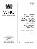
Figures 1-3 presents a series of nonparametric locally weighted regressions, showing the impact
of small-scale weather shocks on child HAZ-scores, on (log) food PCCE and on household food
budget shares
10
. Figure 1A and 1B plots child HAZ-score as a function of (log) total PCCE and
(log) food PCCE, splitting the sample by exposed and unexposed households. Both graphs show
a positive relationship between household PCCE and child nutritional status, with child HAZ-
scores increasing as household total PCCE and total food PCCE increases. However, across the
entire PCCE distribution, the HAZ-scores of children exposed to small-scale weather shocks are
lower than the HAZ-scores of unexposed children. The gap between the ‘exposed’ and
‘unexposed’ lines is indicative of the magnitude of the impact of weather shocks on child
nutritional status and a widening of the gap between the two lines going up the (log) total PCCE
distribution is indicative of a differential impact of small-scale weather shocks at different

10
These plots are obtained using the pooled sample across both years.


16

quantiles. The gap between the two lines is greatest at higher quantiles, suggesting a greater
impact of weather shocks on wealthier households
11
. A similar positive relationship is observed
between child HAZ-score and the consumption of micronutrient-rich food (Figure 1D), while
no clear relationship is observed between child nutritional status and PCCE on energy-rich food
(Figure 1C), suggesting a more important role of micronutrient-rich food in predicting
nutritional status.

Figure 1 HAZ-scores and household consumption: exposed vs. unexposed households

Given the positive relationship between the quality of food and child HAZ-score, lower HAZ-
scores in exposed children is likely to be due to a reduction in household food PCCE,
particularly PCCE on high-nutrient food. Figure 2 and 3 presents nonparametric Engel curves
showing differences between exposed and unexposed households in terms of household budget
share on food (Figure 2A-C) and household (log) food PCCE (Figure 3A-C). Figure 2A-C plots
food budget share as a function of (log) total PCCE, splitting the sample by exposed and
unexposed households. A negative relationship is observed between (log) total PCCE and
household food budget share (Figure 2A) suggesting that food is a necessity for both groups
12
.
However, food budget share in exposed household is lower across the entire distribution of (log)

11
This effect is discussed in more detail in section 5.3 which examines the differential impact of small-scale weather
shocks using parametric modelling.
12
This implies that household PCCE on food grows more slowly than household total PCCE.


17

total PCCE compared to the food budget shares of unexposed households. Similarly, energy-rich
food is a necessity for both groups (Figure 2B), but exposed household allocate a higher
proportion of their food budget to energy-rich food compared to unexposed households. On the
other hand, the share of the food budget allocated to high-nutrient food is lower in the exposed
households compared to unexposed households (Figure 2C) suggesting a reduction in the quality
of dietary intake. Similar results are observed when household (log) food PCCE is plotted as a
function of (log) total PCCE (Figure 3A-C). Compared to unexposed households, exposed

households consume less high-nutrient food and more energy-rich food.

Figure 2 and 3 provides some explanation for the observed differential impact of small-scale
weather shocks on child HAZ-scores at different quantiles of the (log) total PCCE distribution.
The gap in household budget share and (log) PCCE on energy-rich food (Figure 2B and 3B,
respectively) observed between the ‘exposed’ and ‘unexposed’ lines is widest at higher quantiles
of the (log) total PCCE distribution compared to lower quantiles. Similarly, the gap in household
budget share and (log) PCCE on micronutrient-rich food (Figure 2C and 3C), although smaller
than the gap observed with energy-rich food, appears to be larger at the higher quantiles
compared to lower quantiles. This suggests that the differential impact of small-scale weather
shocks on child HAZ-scores may be mediated by the differential impact on the quality of dietary
intake.

Figure 2 Food budget shares in exposed versus unexposed households



18

Differences in parent and household characteristics observed between exposed and unexposed
children (Table 1a) suggests that exposure to small-scale weather shocks are not randomly
distributed. On average, households exposed to small-scale weather shocks are of lower
socioeconomic status compared to unexposed households (Table 1a). For example, compared to
unexposed household, parents in exposed households are less educated, fewer proportions of
households exposed to small-scale weather shocks have access to safe drinking water (64%
versus 71%), flush toilet/septic tank (34% versus 40%) and have larger (log) household sizes
(1.64 versus 1.62). Parental education, access to safe drinking water, and good sanitary conditions
has been shown to be important determinants of child health and nutritional status in developing
countries (Behrman & Deolalikar, 1988; Fewtrell et al., 2005). For example, higher education is
associated with higher income and children with more educated parents are likely to have better

health outcomes compared to children with less educated parents
13
. The following sub-sections
present results of the parametric analyses that accounts for differences in observable
characteristics between exposed and unexposed children.

Figure 3 Food expenditure in exposed versus unexposed households



13
Currie (2009) provides an excellent review of the literature on child health and parental socioeconomic status.


19

5.1 Impact of small-scale weather shocks on child nutritional status

The parametric strategy adopted here estimates the impact of small-scale weather shocks on
child HAZ-scores controlling for observable characteristics correlated with both exposure to
small-scale weather shocks and child HAZ-scores. Exposure to small-scale weather shocks is
assumed to be randomly distributed amongst households living within the same community,
conditional on observable parent and household characteristics. Two community fixed effect
models are specified to test this assumption; the first excludes parent and household
characteristics and the second accounts for parent and household characteristics. Table 2 shows
results of the parametric estimation of the impact of small-scale weather shocks on child HAZ-
scores. In the first specification (first column, Table 2), after controlling for only child
characteristics, HAZ-score of children exposed to small-scale weather shocks are on average
approximately 0.15 standard deviations lower than those of unexposed children. This finding is
consistent with other studies that have reported similar estimates of the impact of small-scale

weather shocks on child nutritional status (Datar et al., 2011; Pörtner, 2010).

An indication of the magnitude of this impact can be deduced using the World Health
Organisation (WHO) growth reference charts
14
which shows corresponding height differences
(comparable to the US NCHS sample) for a given age and gender for a one standard deviation in
HAZ-scores. For example, a one standard deviation in the HAZ-score of a 4 year old male child
is equivalent to a 4.25cm difference in height. Similarly, for a male child aged 8, 12 and 16 year
old, the equivalent height difference is approximately 6.25cm, 6.75cm and 7.5cm, respectively.
Equivalent approximations for girls of similar ages (i.e. 4-16years old) are 4cm, 6cm, 6.5cm and
7cm, respectively. Therefore a reduction in HAZ-scores by 0.15 standard deviation is equivalent
to a reduction in height by approximately 0.6 -1.125cm. Given the potential for future catch-up
growth in children who experience temporary growth retardation in childhood (Adair, 1999)
15
,
the functionally small height differences estimated here may disappear in late
childhood/adolescence. However, repeated exposure to shocks, such as small-scale weather
shocks, throughout childhood is likely to impede any catch-up growth that may have occurred in
late childhood or early adolescence (Martorell et al., 1994).



14
These charts are downloadable from the WHO webpage:

15
The potential for future catch-up growth in children has been disputed by some authors. Some examples include
Martorell et al. (1994) and Hoddinott and Kinsey (2001).

20

Table 2 Impact of weather shocks on child HAZ-score

(1)

(2)

(3)

Exposed
-0.146**
(0.0439)
-0.102*
(0.0391)
-0.0775*
(0.0364)
Male
-0.0352
(0.0332)
-0.0436
(0.0341)
-0.0311
(0.0347)
Kinh (Ethnic majority)
0.576**
(0.107)
0.409**
(0.103)

0.242**
(0.0818)
Older cohort
-0.208**
(0.0439)
-0.228**
(0.0446)
-0.201**
(0.0399)
Year=2009
0.189**
(0.0433)
0.0357
(0.0427)
0.0997*
(0.0397)
Safe drinking water


-0.0428
(0.0424)
-0.0303
(0.0371)
Good sanitation


0.155**
(0.0537)
0.106*
(0.0427)

Log household size


-0.0172
(0.0705)
0.00287
(0.0687)
Prop. of children≤6 years


-0.0630
(0.134)
-0.0988
(0.112)
Urban residence


0.232
(0.240)
0.169
(0.324)
Log total PCCE


0.303**
(0.0478)
0.174**
(0.0387)
M No religion

0.0110
(0.0658)
M Height (cm)




0.0525**
(0.00264)
F age >35 years




-0.0334
(0.0559)
F Primary




0.0425
(0.0915)
F Secondary

0.120
(0.0996)
F High School




0.113
(0.126)
F Degree




0.290*
(0.131)
M age>35 years




-0.0467
(0.0436)
M Primary




0.100

(0.0731)
M Secondary




0.123
(0.0742)
M High School




0.224**
(0.0781)
M Degree




0.325**
(0.100)
Constant
-1.749**
(0.104)
-3.375**
(0.325)
-10.72**
(0.488)
PY Observations

4772

4772

4772

+
p < 0.1,
*
p < 0.05,
**
p < 0.01; Cluster-robust standard errors in parentheses. Base
categories: F and M ≤35years for parents’ age, F and M with no education for parents’ education. PY:
Person-years. All models control for community fixed effects.

In the second specification (second column, Table 2), a set of observable household
characteristics are included while the third specification includes the full set of child, household
and parent characteristics (third column, Table 2). If small-scale weather shocks randomly affect
households, the inclusion of observable household and parent characteristics should have little
or no effect on the magnitude of the estimated impact of small-scale weather shocks on child
HAZ-score. After controlling for household characteristics including (log) total household
PCCE, household size, access to safe drinking water and good sanitation, the magnitude of the
estimated effect of small-scale weather shocks on child HAZ-scores reduces slightly to
approximately 0.1 standard deviations. The inclusion of parent characteristics further reduces the
magnitude of the estimated impact.

The reduction in the magnitude of the impact of small-scale weather shocks suggest that small-
scale weather shocks are disproportionately distributed amongst those whose observed

21

characteristics are correlated with a higher probability of malnourishment, resulting in an
overestimation of the impact of small-scale weather shocks of child nutritional status. For
example, consistent with the literature on child health and parental education, higher parental
education is associated with higher child HAZ-scores (Table 2). Since exposed children, on
average, have parents with lower levels of education (Table 1a), the reduction in the magnitude
of the estimated impact of small-scale weather shocks after controlling for parents education
suggests that part of this impact can be explained by the impact of parent education on child
HAZ-scores. Overall, the estimated impact of small-scale weather shocks on child nutritional
status remain statistically significant after controlling for the full set of child, parent and
household characteristics.

5.2 Impact of small-scale weather shocks on household consumption

The second part of the empirical analysis estimates the impact of small-scale weather shocks on
household consumption and expenditure. Consistent with the literature on child health and
parental socioeconomic status (Cameron & Williams, 2009; Case et al., 2002; Currie, 2009) a
significant positive correlation is observed between child HAZ-scores and household (log) total
PCCE. An increase in household (log) total PCCE is associated with an increase in child HAZ-
scores (Table 2). Similar effects on child HAZ-scores are observed with (log) food PCCE and
(log) micronutrient-rich food PCCE (results shown in Table A1 of the Appendix). Although
energy-rich food has a positive effect on child HAZ-scores, the magnitude of this effect is
considerably less and estimated with less precision, compared to the effect of micronutrient-rich
food on child HAZ-scores
16
. The greater effect of high-nutrient food on child nutritional status
is unsurprising given that micronutrients are more important for maintaining normal body
physiological functions and micronutrient deficiencies could result in higher rates of infection
and stunting as well as higher mortality rates in children (Black et al., 2008; Dewey & Begum,

2011).

Table 3 shows that exposure to small-scale weather shocks is associated with a statistically
significant reduction in (log) total PCCE as well as a reduction in (log) food PCCE (although
statistically insignificant). Differences in the magnitudes of the impact on household (log) total
PCCE and on (log) food PCCE (9 vs. 2 percent) suggest that although small-scale weather
shocks are associated with a reduction in the overall consumption, exposed households appear to
protect food consumption.

16
The full results are shown in Table A1 of the Appendix.


22

Table 3 Impact of weather shocks on household consumption and budget share on food

Log Per Capita Consumption& Expenditure on:

Budget Share on food:
Explanatory Variables
Total PCCE
Total Food
Energy-rich
Nutrient-rich

Total Food
Energy-rich
Nutrient-rich
Exposed

-0.0907**
-0.0161
0.0549*
-0.0569**

-0.00311
0.0213**
-0.0137**

(0.0194)
(0.0154)
(0.0232)
(0.0203)

(0.00746)
(0.00602)
(0.00498)
Log total PCCE
-
0.753**
0.235**
0.880**

-0.107**
-0.127**
0.0652**

-
(0.0195)
(0.0273)

(0.0292)

(0.00735)
(0.00693)
(0.00865)
H Primary
‡‡

0.247**
0.0217
0.0286
0.0641+

0.00223
-0.0131
0.0110

(0.0316)
(0.0218)
(0.0432)
(0.0330)

(0.0119)
(0.0103)
(0.00876)
H Secondary
0.419**
0.00859
0.00245
0.0778*

-0.00728
-0.0184+
0.0220*

(0.0355)
(0.0209)
(0.0422)
(0.0316)

(0.0117)
(0.0106)
(0.00947)
H High School
0.536**
-0.00735
-0.0384
0.0961**

-0.0207
-0.0265*
0.0352**

(0.0351)
(0.0229)
(0.0461)
(0.0306)

(0.0124)
(0.0118)

(0.00981)
H Degree
0.790**
0.0158
-0.0788
0.149**

-0.0123
-0.0310*
0.0523**

(0.0503)
(0.0278)
(0.0479)
(0.0390)

(0.0135)
(0.0116)
(0.0119)
H age >35 years
‡

-0.0466+
0.105**
0.139**
0.1000**

0.0450**
0.00584+
-0.00150

(0.0233)
(0.0158)
(0.0217)
(0.0166)

(0.00676)
(0.00332)
(0.00312)
H Gender (Female)
0.0364
-0.0144
-0.0552+
-0.0318

-0.00778
-0.00350
-0.00248

(0.0363)
(0.0181)
(0.0278)
(0.0239)

(0.00871)
(0.00600)
(0.00675)
Prop. of children≤6years
-0.373**
0.262**

-0.393**
0.574**

0.145**
-0.160**
0.153**

(0.0537)
(0.0446)
(0.0562)
(0.0613)

(0.0191)
(0.0123)
(0.0174)
Log household size
-0.302**
-0.473**
-0.555**
-0.462**

-0.214**
-0.0137*
0.00654

(0.0335)
(0.0227)
(0.0292)
(0.0236)

(0.00992)
(0.00579)
(0.00618)
Urban residence
0.260
-0.0874+
-0.0978
-0.0546

-0.0550**
-0.000794
0.00941

(0.160)
(0.0454)
(0.0696)
(0.0750)

(0.0156)
(0.0220)
(0.0199)
Year=2009
0.394**
-0.104**
-0.141**
-0.100**

-0.0705**
-0.0131*
-0.00684

(0.0231)
(0.0160)
(0.0242)
(0.0211)

(0.00835)
(0.00605)
(0.00874)
Constant
5.922**
1.620**
3.546**
0.00283

1.580**
1.103**
0.0644

(0.0670)
(0.130)
(0.180)
(0.180)

(0.0502)
(0.0434)
(0.0511)
PY Observations
4772
4772

4772
4772

4772
4772
4772
+
p < 0.1,
*
p < 0.05,
**
p < 0.01; Cluster-robust standard errors in parentheses. Base categories:
‡
H ≤35years,
‡‡
H no education. PY: Person-years.


23

Disaggregating food consumption into consumption of micronutrient- and energy-rich foods
shows that exposed households are able to protect total food consumption by reducing the
consumption of high-nutrient food and increasing the consumption of energy-rich food. Similar
results are observed with the impact of weather shocks on household allocation of the food
budget to high-nutrient and energy-rich food (Table 3, column 5-7). The concomitant decrease
and increase in high-nutrient and energy-rich food respectively, is indicative of poorer dietary
intake, thus providing a strong explanation for lower HAZ-scores in children exposed to small-
scale weather shocks.

5.3 Differential impact of small-scale weather shocks

The nonparametric analyses discussed above suggest that the impact of small-scale weather
shocks is greater amongst children living in wealthier households. In this section, this effect is
further investigated by modelling the impact of small-scale weather shocks using two sub-groups
defined by household (log) total PCCE: children living in households below and above the
sample median (log) total PCCE.

Similar to the results seen with nonparametric modelling, small-scale weather shocks has a higher
impact on the stature of children living in wealthier households compared to children from
poorer households (Table 4, column 1). Table 4 (columns 2-6) also provides some explanation
for this observed differential impact and shows that the impact of weather shocks on household
(log) total PCCE is greater in households above the median compared to household below the
median (approximately 8 percent vs. 2 percent). Although the impact on the quantity of food
consumed (log food PCCE) is approximately similar for both sub-groups, the impact on the
quality of food is greater in households above the sample median. In both sub-groups, exposure
to weather shocks is associated with approximately similar magnitudes of reduction in the
consumption of high-nutrient food. However, compared to households below the median, in
households above the median, exposure to weather shocks is associated with a higher increase in
the consumption of energy-rich food (7 percent vs. 3 percent).

As alluded to in section 3.3, the impact of small-scale weather shocks may depend on households
coping strategies or the availability of credit or savings to smooth consumption. This means that
wealthier households may be better equipped to cope with the aftermath of small-scale weather
shocks, thereby, resulting in a lower impact on child nutritional status. For example, Hoddinott
and Kinsey (2001) showed that exposure to droughts adversely affects the height of only


24

children living in poorer households possessing fewer livestock holdings, with no significant

effect on the height of children living in wealthier households. However our results suggest that
wealthier households are not better able to compensate the adverse effects of small-scale weather
shocks and experience greater reductions in household (log) total PCCE as well as in the quality
of dietary intake and hence, lower child HAZ-scores.

This result should be interpreted with caution given the pro-poor sampling strategy adopted by
the VYLS resulting in a sample largely consisting of poorer households compared to a nationally
representative sample
17
. For example, in a nationally representative sample such as the Vietnam
Household Living Standard Survey (VHLSS), average household monthly total PCCE in 2006,
2008 and 2010
18
was estimated at 511, 792 and 1,211 thousand Vietnamese Dong (VND),
respectively (Vietnam General Statistics Office, 2010). Estimates from this study sample are 546
and 817 thousand VND in 2006 and 2009 respectively for household above the sample median
(log) PCCE and 207 and 327 thousand VND, respectively for household below the median.
Thus, ‘wealthier’ households within the VYLS are unlikely to be true representatives of an
average (in terms of a national average) rich household and therefore may not truly reflect the
ability of wealthier households to smooth consumption following weather-induced income
shocks.

On the other hand, failure to observe a significant impact of small-scale weather shocks on the
nutritional status of children from poorer households within this study, may be a reflection of
the wider adverse environmental and living conditions to which children from poorer
households are exposed, which may in turn, pose more risks to child health.

Taken together, this may explain the higher impact of small-scale weather shocks on children
living in ‘wealthier’ households compared to those living in poorer households. Although direct
extrapolations on the heterogeneity of the impact of small-scale weather shocks cannot be made

to a nationally representative sample, this result further strengthens the main findings of this
study on the mechanisms through which small-scale weather shocks affect child HAZ-scores.

17
Nguyen (2008) compares the VYLS to two nationally representative samples: the VHLSS and the Demographic
Health Survey (DHS). Average household wealth index is significantly lower in the VYLS compared to the VHLSS
and the DHS (Nguyen, 2008).
18
No survey was conducted in 2009.