Proceedings VCM 2012 34 Nghiên Cứu Phân Tích Động Lực Học và Ứng Dụng Giải Thuật Di TruyềnLeo Đồi Trong Việc Tối Ưu Hóa Vận Tốc Di Chuyển Thẳng Của Robot Cá 3 Khớp Dạng Carangiform

246 Tuong Quan Vo


VCM2012
Nghiên Cứu Phân Tích Động Lực Học và Ứng Dụng Giải
Thuật Di Truyền-Leo Đồi Trong Việc Tối Ưu Hóa Vận Tốc Di
Chuyển Thẳng Của Robot Cá 3 Khớp Dạng Carangiform
A Study on Dynamic Analysis and Straight Velocity
Optimization of 3-Joint Carangiform Fish Robot Using
Genetic-Hill Climbing Algorithm
Tuong Quan Vo
Ho Chi Minh City, University of Technology – Viet Nam
e-Mail: or
Tóm tắt
Robot phỏng sinh học là một dạng robot mới đã và đang được phát triển trong những năm gần đây. Một số
robot phỏng sinh học đầu tiên được nghiên cứu là robot nhện, robot rắn, robot bò cạp, robot gián,…Trong thời
gian gần đây, hai dạng robot phỏng sinh học hoạt động dưới nước đang được quan tâm nghiên cứu là robot rắn
và robot cá.
Đầu tiên bài báo này giới thiệu về robot cá có 3 khâu, 4 khớp dạng Carangiform. Sau đó, bài báo sẽ giới
thiệu việc áp dụng giải thuật di truyền và giải thuật leo đồi để tối ưu hóa vận tốc di chuyển thẳng cho robot cá.
Đầu tiên, giải thuật di truyền được sử dụng để tạo ra bộ thông số đầu vào tối ưu cho robot cá. Sau đó, bộ thông
số đầu vào này lại được tối ưu một lần nữa bằng giải thuật leo đồi nhằm đảm bảo bộ thông số điều khiển này
gần với kết quả tối ưu toàn cục của hệ thống. Cuối cùng, chúng tôi sử dụng chương trình mô phỏng để kiểm tra
tính đúng đắn của giải thuật đã nêu.
Abstract
Biomimetic robot is a new trend of researched field which is developing quickly in recent years. Some of
the first researches on this field are spider robot, snake robot, scorpion robot, cockroach robot, etc. Lately, two
new types of underwater biomimetic robot called fish robot and snake robot are mostly concerned.
In this paper, firstly a dynamic model of 3-joint (4 links) Carangiform fish robot type is presented.
Secondly fish robot’s maximum straight velocity is optimized by using the combination of Genetic Algorithm
(GA) and Hill Climbing Algorithm (HCA) with respect to its dynamic system. GA is used to create the initial

optimal parameters set for the input functions of the system. Then, this set will be optimized again by using
HCA to be sure that the last optimal parameters set are the global optimization result. Finally, some simulation
results are presented to prove the proposed algorithm.
Keywords - fish robot, dynamic, optimization, GA, HCA, maximum straight velocity, input torque functions.
1. Introduction
Generally, many researches about underwater
propulsion mainly depend on the use of propellers
or thruster to generate the motion for object in
underwater environment. Besides, most of the
natural solutions use the change of object’s body
shape for movement. This changing shape
generates propulsion force to make the object
moves forward or backward effectively.
Carangiform fish robot type is also one kind of the
changing body shape to create the motion for itself
in the underwater environment.
George V. Lauder and Eliot G. Drucker made the
thorough surveys and analyses about motion
mechanisms of fish fin in advance in order to
develop such a successful underwater robot system
[1]. M. J. Lighthill also surveyed about the
hydromechanics of aquatic animal propulsion
because of many kinds of underwater animal
whose motion mechanisms were evolved
throughout many generations to adapt to the harsh
of underwater environment [2]. Based on natural
movement, there are some other researches about
this type of motion. Junzhi Yu and Long Wang
calculated the optimal link ratio of 4-link fish
robot by using computer simulation and he showed

the simulation results by comparing the moving
speed by two cases of models. One is modeled by
Tuyển tập công trình Hội nghị Cơ điện tử toàn quốc lần thứ 6 247


Mã bài: 52
using the optimal link ratio and the other one is
considered without the optimal link ratio [3].
However, most of the researches about fish robot
are based on quite simplified model of fish as well
as experimental approaches. In our research, we
considered a 3-joint (4 links) Carangiform fish
robot type. The dynamic model of the robot is
derived by using Lagrange method. The influences
of fluid force to the motion of fish robot are also
considered which is based on M. J. Lighthill’s
Carangiform propulsion [4]. Besides, the SVD
(Singular Value Decomposition) algorithm is also
used in our simulation program to minimize the
divergence of fish robot’s links when simulating
fish robot’s operation in underwater environment.
The main goal of this paper is the optimization
method to maximize straight velocity of a 3-joint
Carangiform fish robot in x direction. The straight
velocity of fish robot is considered by applying
optimal input torque functions to its dynamic
model. The optimal input torque functions are
gotten by optimized the parameters which are used
to build these functions. Our proposed method to
solve this optimization problem is the combination

of GA and HCA with respect to fish robot’s
dynamic model and some other related constraints.
This combination of GA-HCA gives better results
than our previous work [5]. Another solution for
optimization was proposed by Keehong Seo et al
[6]. They used the numerical optimization
software (NLPP – Non Linear Path Planning –
Tool Box for Matlab) to optimize the control
parameters for a simplified planar model of a
Carangiform fish robot.
2. Dynamics Analysis and Motion Equations
In our fish robot, we focus mainly on the
Carangiform fish’s type because of fast swimming
characteristics which resemble to tuna or
mackerel. The movement of this Carngiform fish
type requires powerful muscles that generate side
to side motion of the posterior part (vertebral
column and flexible tail) while the anterior part of
the body remains relatively in motionless state as
seen in Fig. 1.
Increasing size of movement
Pectoral fin
Posterior partAnterior part
Caudal fin
Tail fin
Main axis
Transverse axis

Fig. 1 Carangiform fish locomotion type.
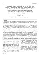
We design 3-joint (4 links) fish robot in order to

get smoother and more natural motion. As
expressed in Fig. 2, the total length of fish robot is
about 600mm which includes 4 links. The head
and body of fish robot are supposed to be one rigid
part (link0) which is connected to link1 by active
DC motor1 (joint1). Then, link1 and link2 are
connected by active DC motor2 (joint2). Lastly,
link3 (lunate shape tail fin) is jointed into link2
(joint3) by two extension flexible springs in order
to imitate the smooth motion of real fish. The
stiffness value of each spring is about 100Nm.
Total weight of the fish robot (in air) is about 4 kg.
l0
(link0)
(link3)
(link2)
(link1)
1
T1
m1 (x1,y1)
Y
X
a1
l1
l2
a2
l3
a3
2
3

m2 (x2,y2)
m3 (x3,y3)
T2

Fig. 2 Fish robot analytical model.
In Fig. 2, T
1
and T
2
are the input torques at joint1
and joint2 which are generated by two active DC
motors. We assume that inertial fluid force F
V
and
lift force F
J
act on tail fin only (link 3) which is
similar to the concept of Motomu Nakashima et al
[7]. The expression of forces distribution on fish
robot is presented in Fig. 3 below. F
F
is the thrust
force component at tail fin, F
C
is lateral force
component and F
D
is the drag force effecting to the
motion of fish robot. The calculations of these
forces are similar to Motomu Nakashima et al

method for their 2-joint fish robot [7].
F
C
V
F
J
F
F
F
F
D
Direction of movement
X
Y

Fig. 3 Forces distribution on fish robot.
We suppose that the tail fin of fish robot is in a
constant flow U
m
so we can derive the inertial
fluid force and the lift force act on the tail fin of
fish robot. Then we can calculate their thrust
component F
F
and lateral component F
C
from the
inertial fluid force and lift force. We also suppose
that the experiment condition of testing our fish
robot is in tank so that the value of U

m
is chosen as
0.08m/s. F
v
is a force proportional to an
acceleration acting in the opposite direction of the
248 Tuong Quan Vo


VCM2012
acceleration [7]. The calculation of F
V
is expressed
in Eq. (1). The lift force F
J
acts in the
perpendicular direction to the flow and its
calculation as in Eq. (2). In these two equations,
chord length is 2C, the span of the tail fin is L and
 is water’s density.
2 2
sin cos
V
F LC U LC U
pr a pr a a
 


(1)
2

2 sin cos
J
F LCU
pr a a

(2)
These fluid force and lift force are divided into
thrust component F
F
in x direction and lateral force
component F
C
in y direction as presented in Fig. 4.

UU
Y
X
F
FV
V
F
CV
F

J
F
Y
X
F
CJ

FJ
F
 

Fig. 4 Model of inertial fluid force and lift force.
In Fig. 4, U is the relative velocity at the center of
the tail fin,  is the attack angle. Based on Fig. 4,
the value of F
F
and F
C
can be calculated by these
two Eqs. (3)-(4):




 


0
1 2 3
0
1 2 3
sin 360
sin 360
F FV FJ V
J
F F F F
F

q q q
q q q
      
   
(3)




 


0
1 2 3
0
1 2 3
cos 360
cos 360
C CV CJ V
J
F F F F
F
q q q
q q q
      
   
(4)
The above two equation can be simplified as
follows:





1 2 3 1 2 3
sin sin
F V J
F F F
q q q q q q
      
(5)




1 2 3 1 2 3
cos cos
C V J
F F F
q q q q q q
     
(6)
If we just consider the movement of fish robot in x
direction, so the relative velocity in y direction at
the center of tail fin is calculated by Eq. (7).







 
1 1 1 1 2 2 1 2
1 2 3 3 1 2 3
cos cos
cos
u l l
a
q q q q q q
q q q q q q
    
    
  
  
(7)
Since U
m
and u are perpendicular as in Fig. 5(a),
so the value of U can be calculated by Eq. (8):
2 2 2
m
U U u
  (8)




u
Um
U
U (b)(a)

Fig. 5 (a) Relationship between U and U
m
. (b)
Diagram of attack angle

calculation.
By using Lagrange’s method, the dynamic model
of fish robot is described briefly as in Eq. (9).
11 12 13 1 1
21 22 23 2 2
31 32 33 3 3
M M M N
M M M N
M M M N
q
q
q
 
   
 
   
 
   

 
   
 
   
 

   
 



(9)
By solving Eq. (9) above, we can get the value of
i
q
,
i
q

(i = 1  3). However, based on the dynamic
model in Eq. (9), SVD (Singular Value
Decomposition) algorithm is also used in our
simulation program to minimize the divergence of
the oscillation of fish robot’s links when
simulating the operation of fish robot in
underwater environment. This divergence also
cause the velocity of fish robot be diverged too.
The motion equation of fish robot is expressed in
Eq. (10).
G
x

is the acceleration of fish robot’s
centroid position.
m
is the total weight of fish

robot in water (
11.45
m

kg). F
F
is the propulsion
force to push fish robot forward and F
D
is drag
force caused by the friction between fish robot and
the surround environment when fish robot swims.
G F D
mx F F
 
 


(10)
The calculation of F
D
is presented in Eq. (11)
2
1
2
D D
F V C S
r (11)
Where
r

is the mass density of water.
V
is the
velocity of fish robot relative to the water flow.
D
C
is the drag coefficient which is assumed to be
0.5 in the simulation program.
S
is the area of the
main body of fish robot which is projected on the
perpendicular plane of the flow


2
0.021
S m
 .
3. Velocity Optimization Method
3.1 Genetic Algorithm (GA) and Hill Climbing
Algorithm (HCA)
Genetic Algorithm [8] [9] is based on the process
of Darwin’s theory of evolution by starting with a
set of potential population with some or many
individuals and then changing them during several
iterations. The first potential population is
generated or selected randomly or arbitrary. The
individual in the population is called chromosome.
The entire set of these chromosomes is called
population. The chromosomes evolve during

several iterations called generations. GA uses the
concept of survival of the fitness by randomly
initializing a population of individual in which
each individual contains the parameters to reach to
Tuyển tập công trình Hội nghị Cơ điện tử toàn quốc lần thứ 6 249


Mã bài: 52
a possible solution of an optimization problem.
Each individual in the population is assigned a
fitness value that is used to indicate the quality of
the individual as an optimal solution for the
problem or not. Then, the selected individuals
become parents based on their fitness value and
then continue to create the next generation of the
potential solution to the optimal problem. The new
potential generations are generated using the
methods of crossover and mutation.
Sometimes, the result of GA is just the local
optimum. It is not the global optimal solution for
the whole problem. In this case, we use HCA to
optimize the result of GA again to make this result
better. Besides, the optimization by HCA will also
find the global optimal solution for the problem.

Y
X
Global maximum
Local m axim um
Flat local maxim um

Beginning Position

Fig. 6 Hill climbing demonstration.

However, there are two popular combinations
between these two algorithms such as: HCA-GA,
GA-HCA. The first type of combination (HCA-
GA) was used in our previous work [5] which
gave worse result than the second combination
(GA-HCA) as introduced in this paper. HCA [10]
[11] is one of the effective methods to find the
global optimum of a problem. The conceptual
diagram of HCA can be seen in Fig. 6. The
process of HCA can be expressed by the following
steps:
Step 1: Pick a random point in the search space.
Step 2: Consider all the neighbors of the current
state.
Step 3: Choose the neighbor with the best quality
and move to that state.
Step 4: Repeat Step 2 to Step 4 until all the
neighboring states are of lower quality.
Step 5: Return the current state as the solution of
the problem.
3.2 Using GA-HCA to maximize the straight
velocity of fish robot
The general algorithm diagram of the optimal
problem is introduced in Fig. 7.
Fish robot has two active joints that are joint1 and
joint2 to generate the movement for whole robot.

Two input torque functions equations which
support for joint1 and joint2 as T1 and T2 in Fig. 2
are calculated as in Eqs. (12)-(13):


1 1 1
sin 2
T A f t
p

(12)


2 2 2
sin 2T A f t
p b
 
(13)
1 2
,
A A
: Amplitude of input torques for motor 1, 2 .
1 2
,
f f
: Frequency of input torques for motor 1, 2.
b
: Phase angle between input torques of two
motors.
From two Eqs. (12)-(13), there are five parameters

1 2 1 2
, , , ,
A A f f
b
need to be optimized to build two
input functions
1
T
and
2
T
for the system.

Fig. 7 General algorithm of the optimization
problem.

The propulsive speed of fish robot in steady state
is presented by Eq. (14):
F
P
F
h
u  (14)
h
: Propulsive efficiency


0.4
h


.
P
: Average consumed power.
1 1 2 2
2
T T
P
q q


 

In GA and HCA, fitness function is used to
evaluate the suitable parameters’ value for the
system. The main ideas of fitness function for GA
and HCA is: maximum propulsive speed gives
maximum velocity of fish robot. Besides, the
250 Tuong Quan Vo


VCM2012
algorithm of this fitness function is also based on
the dynamic model of fish robot in order to check
the suitability of these parameters to the fish robot
or not. The algorithm of fitness function is
expressed in Fig. 8.
21
,




F
F
P



F
ig. 8 Fitness function of GA-HCA.
In order to use the optimization method by GA-
HCA, it requires 6 constraints criteria of the
optimized parameters as expressed in Eq. (15)
below:
1
2
1
2
0 0
1. 0 5
2. 0 5
3. 0 2
4. 0 2
5. 0 60
6. Dynamic model of fish robot
A
A
f
f
b
 

 
 
 
 
(15)
The role of HCA is used to find the global optimal
values of parameters set which is based on the
population of parameters set generated by GA and
fitness function. HCA algorithm is expressed by
Fig. 9 below.

Fig. 9 HCA
By using GA, if the result is the real optimal one,
it will keep in similar values in many next
generations. We can depend on this characteristic
of GA to make the stop condition for the
optimized process.
3.3 GA-HCA implementation
The simulation results of the algorithms in this
paper are carried out by using Matlab program
with the toolbox of GA [12]. The GA simulation
program runs with the population of 500 and the
generation of 500. During the heredity process, we
use the selection method as normalized geometry
select, the multi-non-uniform mutations as the
mutation method and the arithmetic crossover as
the crossover method. Then, the optimal
population generated by GA will be optimized by
HCA to be sure that the last optimal parameters set
is the global optimal set for the system.

Besides, in order to prove the effective of this
proposed optimization method we also carried out
the survey about the behavior of fish robot
velocity which input torque functions’ parameters
set are chosen arbitrary (arbitrary case). Normally,
there is no method to choose the suitable values of
Tuyển tập công trình Hội nghị Cơ điện tử toàn quốc lần thứ 6 251


Mã bài: 52
a five parameters set of
1 2 1 2
, , , ,
A A f f
b
to build two
input torque functions for the system. Besides, the
range value of each parameter in the set also does
not know exactly. By surveying the relationship
between velocity and each parameter in the set, we
know the divergent range of velocity value. So,
base on this result we can choose suitable the
range value of each parameter for the optimal case
as expressed in Eq. (15). Actually in arbitrary case,
we can also base on this survey to choose the
parameters’ value for the system which relies on
their range. However, this is not an optimal
method because if one of the values in the set is
chosen unsuitable, these input functions will make
the system halt or divergence. Or we can choose

the most maximum parameters for the input
functions to create the maximum velocity for fish
robot. This method is also not good because the
maximum value of parameters set can also be
harmful to the mechanism structure of fish robot.
Therefore, by using the optimal algorithm by GA-
HCA, the combination values of these five
parameters
1 2 1 2
, , , ,
A A f f
b
are chosen and
evaluated suitably to be sure that those values will
make fish robot swim at the maximum velocity.
Moreover, by comparison our optimal results done
by simulation method with other results carried out
by experiment method of other researchers, the
advantage of our proposed methods can be proved.

4. Simulation Results
4.1 Survey the influence of input torque
functions’ parameters to the velocity of fish
robot
The influences of those parameters to fish robot
velocity are considered by observing the relation
graphs between velocity and those parameters. In
these cases, we consider the behavior and velocity
value of fish robot with respect to amplitudes (A
1

,
A
2
), frequencies (f
1
, f
2
), or phase angle .
4.1.1 The relationship between fish robot
velocity and amplitudes
In order to survey this relation, the values of
amplitude A
1
, A
2
are changed while the value of
frequencies and phase angle are kept as constants.
Then we input some different input functions pairs
which are built by this rule to the dynamic model
of fish robot to consider the behavior of its
velocity as presented in Fig. 10. In Fig. 10 the
value of f
1
= f
2
= 0.2Hz and  = 30
0
are kept as
constants.
0 1 2 3 4 5 6 7 8 9 10

0
0.1
0.2
0.3
0.4
0.5
0.6
0.7
0.8
The relationship between amplitude and velocity - Beta = 30 Degree, f1 = f2 = 0.2 Hz
Time (s)
Velocity of fish robot(m/s)


A1 = A2 = 1 Nm
A1 = A2 = 2.5 Nm
A1 = A2 = 3.5 Nm
A1 = A2 = 4.5 Nm
A1 = A2 = 5 Nm

(a)

0 1 2 3 4 5 6 7 8 9 10
0
2
4
6
8
10
12

14
16
18
The relationship between amplitude and velocity - Beta = 30 Degree, f1 = f2 = 0.2 Hz
Time (s)
Velocity of fish robot(m/s)


A1 = A2 = 5.5 Nm


(b)
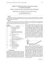
Fig. 10 (a) The relationship between amplitudes
and velocity with f
1
= f
2
= 0.2Hz,

= 30
0
. (b)
Divergence case.
In Fig. 10(a), when A
1
= A
2
= 5Nm (the topmost
continuous line), velocity of fish robot has the
trend to be diverged. So, if the amplitudes A

1
and
A
2
are increased to over 5Nm (for example 5.5
Nm), the velocity will be diverged as expressed in
Fig. 10(b). Besides, in Fig. 10(a), the performance
of velocity has big oscillation when amplitude
values reach to 5Nm. Therefore, we can choose
the value of amplitudes be smaller or equal than
5Nm. And the value of amplitudes equal to 5Nm
can be called the limited amplitude of divergence
in this case.
0 1 2 3 4 5 6 7 8 9 10
0
1
2
3
4
5
6
The relationship between amplitude and velocity - Beta = 30 Degree, f1 = f2 = 0.6 Hz
Time (s)
Velocity of fish robot (m/s)


A1 = A2 = 0.5 Nm
A1 = A2 = 1 Nm
A1 = A2 = 2 Nm
A1 = A2 = 3 Nm

A1 = A2 = 4 Nm

Fig. 11 The relationship between amplitudes and
velocity, f
1
= f
2
= 0.6Hz,

= 30
0
.
In next example, we increase the value of
frequencies to 0.6Hz and keep phase angle’s value
does not change to consider the behavior of this
relationship. In Fig. 11 above, with the value of f
1
252 Tuong Quan Vo


VCM2012
= f
2
= 0.6Hz and  = 30
0
, if amplitude values are
greater than 4Nm (the topmost dash line) the
velocity will have the trend to be diverged. So, the
amplitudes value equal to 4Nm can also be called
the limited amplitude of divergence in this case.

Generally, from two Figs. 10-11, if frequencies are
increased, the amplitudes need to be decreased to
keep the velocity of fish robot not diverges.
Moreover, bigger amplitude also makes bigger
velocity of fish robot.
4.1.2 The relationship between fish robot
velocity and frequency
Similar to previous case, to survey about the
relationship between frequency and velocity, we
keep the values of amplitudes and phase angle are
constants while changing the value of frequencies
to consider the performance of fish robot velocity
as expressed in Fig. 12.
In Fig. 12(a), the velocity has trend to be diverged
when f
1
= f
2
= 0.7Hz (the top dash dot line) or f
1
=
f
2
= 0.9Hz (the topmost dash line). So, if
frequencies’ value are greater than 0.9Hz (for
example 0.98Hz), the velocity will be diverged as
expressed in Fig. 12(b). Therefore, 0.98Hz can be
said to be the limited frequency of divergence in
this case.
0 1 2 3 4 5 6 7 8 9 10

0
0.2
0.4
0.6
0.8
1
1.2
1.4
The relationship between frequency and velocity - A1 = A2 = 3 Nm, Beta = 30 Degree
Time (s)
Velocity of fish robot (m/s)


f1 = f2 = 0.1 Hz
f1 = f2 = 0.3 Hz
f1 = f2 = 0.5 Hz
f1 = f2 = 0.7 Hz
f1 = f2 = 0.9 Hz

(a)
0 1 2 3 4 5 6 7 8 9 10
0
5
10
15
20
25
The relationship between frequency and velocity - A1 = A2 = 3 Nm, Beta = 30 Degree
Time (s)
Velocity of fish robot (m/s)

f1 = f2 = 0.98 Hz

(b)
Fig. 12 (a) The relationship between frequencies
and velocity with A
1
= A
2
= 3Nm,

= 30
0
. (b)
Divergence case.
By reducing the amplitudes value, the divergent
frequency value will be increased as expressed in
Fig. 13. So, with smaller amplitudes value A
1
= A
2
= 1Nm, the velocity of fish robot will be diverged
when frequencies’ value are greater than or equal
1.6Hz (the topmost dash line). Similarly, the value
of 1.6Hz is also called limited frequency of
divergence in this case.
Therefore, in the relationship between frequency
and velocity, the bigger frequency will make the
bigger velocity of fish robot. Besides, frequency

range will be extended when amplitude range is
shrunk.

0 1 2 3 4 5 6 7 8 9 10
0
0.5
1
1.5
2
2.5
3
3.5
4
4.5
The relationship between frequency and velocity - A1 = A2 = 1 Nm, Beta = 30 Degree
Time (s)
Velocity of fish robot (m/s)


f1 = f2 = 0.3 Hz
f1 = f2 = 0.7 Hz
f1 = f2 = 1 Hz
f1 = f2 = 1.4 Hz
f1 = f2 = 1.6 Hz

Fig. 13 The relationship between frequencies and
velocity with A
1
= A
2

= 1Nm,

= 30
0
.

4.1.3 The relationship between fish robot
velocity and phase angle
The phase angle  between two input torque
functions also has big influence to the velocity of
fish robot. The relationship between velocity of
fish robot and phase angle is carried out by
keeping in constant the values of amplitudes (A
1
,
A
2
) and frequencies (f
1
, f
2
). The performance of
velocity based on this relation is expressed by
Figs. 14 below.
Tuyển tập công trình Hội nghị Cơ điện tử toàn quốc lần thứ 6 253


Mã bài: 52
0 1 2 3 4 5 6 7 8 9 10
0

0.02
0.04
0.06
0.08
0.1
0.12
0.14
The relationship between phase angle and velocity - A1 = A2 = 1.5 Nm, f1 = f2 = 0.3 Hz
Time (s)
Velocity of fish robot (m/s)


Beta = 1 Degree
Beta = 10 Degree
Beta = 30 Degree
Beta = 50 Degree
Beta = 60 Degree
0 1 2 3 4 5 6 7 8 9 10
0
0.2
0.4
0.6
0.8
1
1.2
1.4
The relationship between phase angle and velocity - A1 = A2 = 3 Nm, f1 = f2 = 0.7 Hz
Time (s)
Velocity of fish robot (m/s)

Beta = 1 Degree
Beta = 10 Degree
Beta = 30 Degree
Beta = 50 Degree
Beta = 60 Degree

Fig. 14 The relationship between phase angle and
velocity
4.2 Optimal results created by GA-HCA
In this optimization method, the optimal value of
five parameters


1 2 1 2
, , , ,
A A f f
b
will be generated
by GA-HCA simultaneously base on each
parameter’s range values as in Eq. (15). The input
torque functions built by these optimal parameters
will make fish robot swim at the maximum
velocity with respect to its dynamic model. In this
optimization program, we will consider the two
frequencies of two motors are similar


1 2
f f f

 

and it is called same frequencies case. Therefore,
the optimization method will optimize four
parameters


1 2
, , ,
A A f
b
.
Table 1: Optimal value of parameters set by GA-
HCA
A1 A2 f1 = f2 Beta Fitness
1.36 1.38 1.24 14.62 7.46
The two input torque functions for the system are
introduced as Eq. (17)




1
2
1.36sin 2 *1.24
1.38sin 2 *1.24 14.62
T t
T t
p
p


 
(17)
By applying two input torque functions in Eq. (17)
to the dynamic model of fish robot, the average
velocity value of fish robot is about 0.59 (m/s)
during the concerning time of 20 seconds. Fig. 15
simulates the operation of fish robot’s mechanism
system during concerning time in same
frequencies case.
The relationship graph between velocity-time and
moving distance-time of fish robot by inputting
Eq. (17) to the dynamic system are expressed in
Fig. 16 below. In this case, fish robot swims at
distance at about 11.69m after 20 seconds. After
about 14 seconds, velocity of fish robot will be
kept stable at the average value of 0.62 (m/s).
0 5 10 15 20
-20
-10
0
10
20
Link 1
Displacement link1 (theta1) (Degree)
Time (s)
0 5 10 15 20
-4
-2
0

2
4
Link 1
Angular velocity theta1 (rad/s)
Time (s)
0 5 10 15 20
-10
-5
0
5
10
Link 2
Displacement link2 (theta2) (Degree)
Time (s)
0 5 10 15 20
-2
-1
0
1
2
Link 2
Angular velocity theta2 (rad/s)
Time (s)
0 5 10 15 20
-2
-1
0
1
2
Link 3

Displacement link3 (theta3) (Degree)
Time (s)
0 5 10 15 20
-0.2
-0.1
0
0.1
0.2
Link 3
Angular velocity theta3 (rad/s)
Time (s)

Fig. 15 Fish robot links ‘oscillation and their
angular velocities created by using Eq. (17).
0 2 4 6 8 10 12 14 16 18 20
0
5
10
15
The relation between moving distance and time
Time (s)
Moving distance (m)
0 2 4 6 8 10 12 14 16 18 20
0
0.2
0.4
0.6
0.8
The relationship between real velocity and time
Time (s)

Velocity of fish robot (m/s)

Fig. 16 Fish robot velocity and moving distance
with respect to time by using Eq. (17).
In Fig. 16, the velocity of fish robot takes about 12
seconds to reach to the stable state. Or, it can be
said that there is no big change in velocity’s value
after the steady state as in Fig. 16.
Generally, in our proposed method, the optimal
result is generated by GA-HCA. The results of this
method are just the simulations. Our next step is to
carry out some experiment which is based on these
simulation results. Besides, some researchers as
Motomu Nakashima et al [7] and Koichi Hirata et
al [13] used experiment method to find the optimal
velocity for their fish robot. The maximum
velocity of fish robot done by Motomu Nakashima
is about 0.5 (m/s) and Koichi Hirata’s fish robot
velocity is around 0.2 (m/s). By comparison our
proposed method and these two experiment
method of two researchers above, our simulation
results are nearly similar. This means; by using
optimization algorithm by GA-HCA, we know that
254 Tuong Quan Vo


VCM2012
our fish robot will swim at the maximum velocity
at about 0.62 (m/s) in optimal cases.

5. Conclusion
In this paper, a model of 3-joint Carangiform fish
robot type is presented. From this type of fish
robot, its dynamic model is derived by using
Lagrange’s method. Besides, the influence of fluid
force which exerts on the motion of fish robot in
underwater environment is also considered in
robot’s dynamic model by using the concept of M.
J. Lighthill’s Carangiform propulsion. Besides,
SVD algorithm is also used in our simulation
program as an effective method to reduce the
divergence of fish robot links when solving the
matrix of its dynamic model.
By inputting different arbitrary values of input
torque functions T
1
, T
2
to fish robot’s dynamic
system, we made a survey on the relationship
between fish robot velocity and other parameters
of two input functions. For example, some of the
relationships are amplitude-velocity, frequency-
velocity and phase angle-velocity. The results of
this survey are used to define the range value of
each parameter in the input function. Besides,
these ranges of parameters’ value are also the
constraints criteria for the optimization program of
GA-HCA. Then, by using the combination of GA-
HCA simulation program, the optimal parameters

set which are built two input torque functions for
two active motors at joint1 and joint2 are gotten.
These two optimal input torque functions can
make fish robot swim at the maximum velocity at
about 0.62 (m/s) with respect to its dynamic
model.

6. Future works
In continuing to this problem, some experiments
are going to be carried out to check the agreement
between simulation results and the experiment
results. Besides, another control problems will also
considered in the next steps.

References
[1] Lauder, G.V. and Drucker, E.G., Morphology
And Experimental Hydrodynamics Of Fish Fin
Control Surfaces, IEEE Journal of Oceanic
Engineering, Vol. 29, No. 3, pp. 556-571, July
2004.
[2] M. J. Lighthill, Hydromechanics Of Aquatic
Animal Propulsion, Annual Review of Fluid
Mechanics, January 1969, Vol. 1, pp. 413-446
[3] Junzhi Yu and Long Wang, Parameter
Optimization Of Simplified Propulsive Model
For Biomimetic Robot Fish, Proceeding of the
2005 IEEE, International Conference on
Robotics and Automation, Barcelona, Spain, pp.
3306-3311, April 2005.
[4] M. J. Lighthill, Note On The Swimming of

Slender Fish, Journal of fluid mechanics, Vol 9,
pp 305-317, 1960.
[5] Tuong Quan Vo, Byung Ryong Lee, Hyoung
Seok Kim and Hyo Seung Cho, Optimizing
Maximum Velocity of Fish Robot Using Hill
Climbing Algorithm and Genetic Algorithm, The
10
th
International Conference on Control,
Automation, Robotics & Vision, 17-20
December 2008, Hanoi, Vietnam.
[6] Keehong Seo, Richard Murray, Jin S. Lee,
Exploring Optimal Gaits For Planar
Carangiform Robot Fish Locomotion, 16
th
IFAC
World Congress in Prague, 2005.
[7] Motomu NAKASHIMA, Norifumi OHGISHI
and Kyosuke ONO, A Study On The Propulsive
Mechanism Of A Double Jointed Fish Robot
Utilizing Self-Excitation Control, JSME
International Journal, Series C, Vol. 46, No. 3,
pp. 982-990, 2003.
[8] Colin R. Reeves, Jonathan E. Rowe, Genetic
Algorithms – Principles And Perspectives, A
Guide to GA Theory, Kluwer Academic
Publishers, 2003.
[9] Randy L.Haupt, Sue Ellen Haupt, Practical
Genetic Algorithms – Second Edition, A John
Willey & Son, Inc., Publication, May 2004.

[10] Andrew W. Moore, Iterative Improvement
Search Hill Climbing, Simulated Annealing,
WALKSAT, and Genetic Algorithms, School of
Computer Science Carnegie Mellon University.
[11] Masafumi Hagiwara, Pseudo Hill Climbing
Genetic Algorithm (PHGA) for Function
Optimization, Proceeding of 1993 International
Joint Conference on Neural Networks.
[12] Christopher R. Houck, Jeffery A. Joines,
Michael G. Kay, A Genetic Algorithm for
Function Optimization: A Matlab
Implementation, North Carolina State
University.
[13] Koichi HIRATA*, Tadanori TAKIMOTO** and
Kenkichi TAMURA***, Study on Turning
Performance of a Fish Robot, *Power and
Energy Engineering Division, Ship Research
Institute, Shinkawa 6-38-1, Mitaka, Tokyo 181-
0004, Japan, **Arctic Vessel and Low
Temperature Engineering Division, Ship
Research Institute, *** Japan Marine Science
and Technology Center.

Tuyển tập công trình Hội nghị Cơ điện tử toàn quốc lần thứ 6 255


Mã bài: 52
Vo Tuong Quan was born in
1979, Ho Chi Minh City, Viet
Nam. In 2005, he received his

MSE in Ho Chi Minh City
University of Technology, Viet
Nam about Machine Building
Engineering. And, in 2010, he
received his PhD in University
of Ulsan, Ulsan, Korea about
Mechanical and Automotive
Engineering.
He has been a Lecturer in the Department of
Mechatronics, Faculty of Mechanical Engineering,
Ho Chi Minh City University of Technology from
2002 until present. His currently researches are
about the underwater robots, biomimetic robots,
bio-mechatronics systems and automatic control
systems in industry.