Proceedings VCM 2012 76 thiết kế hệ thống nhận dạng khẩu lệnh tiếng việt
Bạn đang xem bản rút gọn của tài liệu. Xem và tải ngay bản đầy đủ của tài liệu tại đây (191.56 KB, 8 trang )
Tuyển tập công trình Hội nghị Cơ điện tử toàn quốc lần thứ 6 559
Mã bài: 129
Communication delay Compensation for NCSs based on AR modeling
Bù trễ truyền thông đối với các hệ thống điều khiển
có nối mạng dựa trên mô hình AR
Nguyen Trong Cac, Nguyen Van Khang
Hanoi University of Science and Technology
e-Mail: ,
Abstract
Communication delay in Networked Control Systems (NCSs) are random in nature. A distributed real-time
control system linked through a communication network is bound to be affected by the randomness of
communication delay patterns. Real time feature in NCSs does not only depend on the real time of each part
but also depends on the flexible links between parts. In time-sensitive NCSs, if the delay time exceeds the
specified tolerable time limit, the plant or the device can either be damaged or have a degraded performance of
system. In order to study the communication delay compensation for NCSs, in this paper Autoregressive (AR)
modeling was proposed. The simulation results for communication delay illustrate that the AR model is able to
compensate for the delay, thus guaranteeing the stability of NCSs in the presence of unpredictable delays.
Keywords: Networked Control Systems; communication delay; Autoregressive modeling.
Tóm tắt
Trễ truyền thông trong các hệ thống điều khiển có nối mạng (NCSs) là ngẫu nhiên trong tự nhiên. Một hệ
thống điều khiển thời gian thực phân tán được liên kết với nhau thông qua một mạng truyền thông bị ràng buộc
bởi ảnh hưởng ngẫu nhiên của các thành phần trễ truyền thông. Tính năng thời gian thực trong NCSs không
chỉ phụ thuộc vào thời gian thực của từng thành phần mà còn phụ thuộc vào sự phối hợp linh hoạt giữa các
thành phần đó. Trong NCSs mà nhạy cảm với thời gian, nếu thời gian trễ vượt quá giới hạn thời gian cho phép
đã được quy định thì nhà máy hoặc các thiết bị có thể bị hư hỏng, làm suy giảm hiệu suất của hệ thống. Để
nghiên cứu bù trễ truyền thông đối với NCSs, trong bài báo này mô hình AR được đề xuất. Các kết quả mô
phỏng minh họa đối với trễ truyền thông cho thấy rằng mô hình AR có thể sử dụng để bù trễ, đảm bảo sự ổn
định của NCSs với sự có mặt của trễ mà không thể dự đoán trước.
Từ khóa: Các hệ thống điều khiển có nối mạng; Trễ truyền thông; mô hình Autoregressive.
1. Introduction
Feedback control systems wherein the control
loops are closed through a real-time network are
called NCSs, The defining feature of a Networked
Control System is that information (reference
input, plant output, control input, etc.) is
exchanged using a network among control system
components (sensors, controller, actuators, etc.)
[1]. Thus a network control system requires at
least one link to be carried by a real-time network
[2]. The most preferred network protocols for
control systems are Ethernet-based Modbus,
Profibus, or Controller Area Network (CAN). The
time delays are not always local to the controller
tasks. They can occur as transmission delays from
a sensor to a controller and from a controller to an
actuator, because control equipment is connected
via network [3]. The communication delay in
NCSs includes three parts [3]: from sensor to
controller
sc
, from controller to actuator
ca
,
falculating time of controller
c
, which is related to
the calculating algorithm (
c
is usually small
enough to be omitted as disturbance). The
sc
and
ca
are caused by the data transfer over the
network. The data transfer in the network has time
stamps, so the
sc
can be easily obtained by
comparing time stamps. However the
ca
can not
be obtained easily and directly.
For the communication delay compensation for
Networked Control System, so far many methods
have been proposed. Different mathematical,
heuristic, and statistical-based approaches are
taken for delay compensation in NCSs [4]. The
optimal stochastic method approaches the problem
as a Linear–Quadratic–Gaussian (LQG) problem
[5]. In [6] focused on the effect of delay jitter at a
fixed mean delay on the quality-of-control, two
sources of delay jitter are identified in EIA-852-
based systems: network traffic induced and
protocol induced. Li et al. [7] derived Linear
Matrix Inequality (LMI)-based sufficient
conditions for stability. Xia et al. [8] proposed a
new control scheme consisting of a control
prediction generator and a network delay
560 Nguyen Trong Cac, Nguyen Van Khang
VCM2012
compensator. In [9] proposed a time delay
compensation method based on the concept of
network disturbance and communication
disturbance observer. In this method, a delay time
model is not needed. Liu [10], [11] proposed a
predictive control scheme for Networked Control
System with random network delay in both the
feedback and forward channels and also provided
an analytical stability criteria for closed-loop
Networked Predictive Control (NPC) systems,
which is a model-based predictive control
algorithm. The plant model must be accurate and it
needs the synchronization of the clocks between
organs. In [12] a new control scheme termed
networked predictive control is proposed. This
scheme mainly consists of the control prediction
generator and network-delay compensator. Hu
[13] proposed a new event-driven NPC scheme.
The control signal applied to the actuator is
selected based on the output rather than on the
time delay measured. This scheme fits in the case
that the model is not accurate or has uncertainty or
disturbance. But the delay compensator is based
on the assumption that the delay
sc
and
ca
, i.e.,
Round Trip Time (RTT) are known.
Communication delay compensation thus has been
studied in depth, and many solutions, some
application-based and some theoretical, are
proposed in the literature. Today, NCSs are
moving into distributed NCSs, which are
multidisciplinary efforts whose aim is to produce a
network structure and components that are capable
of integrating distributed sensors, distributed
actuators, and distributed control algorithms over a
communication network in a manner that is
suitable for real-time applications [14]. In order to
study the communication delay compensation for
NCSs, in this paper Autoregressive (AR) modeling
was proposed. The simulation results for
communication delay illustrate that the AR model
is able to compensate for the delay, thus
guaranteeing the stability of NCSs in the presence
of unpredictable delays.
2. System Design
2.1 System structure
In general, time-delay appears different
characteristic at different time region or under
different network load, the AR modeling method
can better depict this characteristic. So the AR
method is used for
ca
(kT) modeling. Based on the
ca
(kT)
modeling and the assumption that the
model of the plant is prior known, a new time-
delay compensation scheme for NCSs is proposed
as Fig. l.
Fig. 1 Block diagram of new communication delay compensation scheme for NCSs
In the forward channel, there are three parts: The
first part is the controller. The second part is an
identifier for the time delay from the controller to
actuator
ca
(kT), for which we can use the data in
the buffer to build the estimated models. For the
characteristic of
ca
(kT), an AR modeling is
adopted, which is noted as an estimated one
ˆ
( )
i
ca
kT
for each time region. The last part is
networked compensator
ˆ
( ) ( )
i
sc ca
u kT kT kT kT
, which compensates
for the network time-delay and data dropout in the
forward (from controller to actuator) and feedback
(from sensor to controller) channels and achieves
the desired control performance. In the feedback
channel, there is a predictive generator, which
generates an accessorial predictive vector
( ) ( )
sc sc
y kT kT m kT kT
based on the data
( )
sc
y kT kT
in the buffer.
In this scheme, a control cycle is initiated by the
plant side. The plant output side sends a packet to
the controller side, where the previous control
signals u(kT) and previous output y(kT) are
packed together for AR modelling used. When the
controller side receives the packet, based on the
data
( )
sc
y kT kT
received (note that there is a
time-delay
sc
(kT) from the sensor to the
Controller
r(kT)
+
_
ca
(kT)
u(kT)
Identifier
u(kT-
ca
(kT))
Compensator
Plant
Z.O.H
y(t)
T
sc
(kT)
AR
modeling
y(kT)
y(kT-
sc
(kT))
e(kT)
y(kT
-
sc
(kT)+m
kT-
sc
(kT))
Network
u(t)
Tuyển tập công trình Hội nghị Cơ điện tử toàn quốc lần thứ 6 561
Mã bài: 129
controller), it calculates future control sequences
( )
sc
u kT kT
, packs them into a packet together,
and sends it through the network. There is another
time delay
ca
(kT) from the controller to the
actuator. So on the left side of the identifier,
( ) ( )
sc ca
u kT kT kT
is arriving. In the feedback
channel, based on the buffered data
( )
sc
y kT kT
, them-step predictive
( ) ( )
sc sc
y kT kT m kT kT
can be obtained,
which is sent to the identifier also. By using a m-
deep antitheses to get the time-delay
ca
(kT). Here
an AR modeling is built for
ca
(kT) which is noted
as
ˆ
( )
i
ca
kT
for each time region. Then it is packed
to the compensator to combine with other
appropriate methods to compensate the controller
and apply to the actuator. Therefore, the task of the
compensator side is only to generate the correct
control sequence and has no internal states, so it is
not necessarily have to be synchronized with the
plant side.
Different from NPC implementation using the
synchronization requirement and that all the
predictions at the plant side are based on the RTT
delay, the estimator
ˆ
( )
i
ca
kT
is plus here to solve
the puzzle [10-13]. However, in the compensator,
we can use the
ˆ
( )
i
ca
kT
combined with many
control schemes, such as NPC used in Liu and Hu.
2.2 AR modeling
Consider a single-input single-output discrete-time
plant described by the autoregressive moving
average model [13]:
1 1
( ) ( ) ( ) ( 1)
A z y kT B z u kT
(1)
Where u(kT) ,y(kT) are the control input vector
and output vector of the systems at time t.
1 1
( ) [ , ]
A z z n
and
1 1
( ) [ , ]
B z z m
are
polynomials, i.e.,
1 1
0 1
1 1
0 1 0
( ) ,
( ) , 0
n
n
m
m
A z a a z a z
B z b b z b z and a
Without considering the network transmission
delay, a controller is designed as:
1 1
( ) ( ) ( ) ( )
C z u kT D z e kT
(2)
Where
1 1 1 1
( ) [ , ] ( ) [ , ]
c d
C z z n and D z z n
are
polynomials, and c
0
=1.
( ) ( ) ( )
e kT r kT y kT
(3)
Where r(kT) is the reference input.
It is assumed that the feedback channel time delay
is
sc
(kT) which can be measured through the time
stamps in the packages between the output sensor
and the controller. At time t, the controller side
receives a packet from the plant side, including the
sequences of plant output y and the previous
control sequences u, which is noted as:
( ( )), ( ( ) 1), ( ( ) )
( ( ) 1), ( ( ) 2), ( ( ) )
sc sc sc
sc sc sc c
including y kT kT y kT kT y kT kT n
including u kT kT u kT kT u kT kT n
(4)
These data are buffered in a data box. The control
sequence can be predicted as:
1
1
( )
(1 ( )) ( )
( ) ( ( )) ( )
sc sc
sc sc
sc sc sc
u kT kT
C z u kT kT
D z r kT kT y kT kT
(5)
Where
( )
u kT i kT
denotes the ith step-ahead
prediction of u(kT) based on the previous data up
to time t. Then, the m-step system output
prediction is obtained as:
1
1
( ( ) ( ))
1 ( ) ( ( ) ( ))
( ) ( ( ) ( ))
sc sc
sc sc
sc sc
y kT kT m kT kT
A z y kT kT m kT kT
B z u kT kT m kT kT
(6)
Correspondingly, the control signal m-step ahead
prediction is:
1
1
( ( ) ( )) 1 ( ) ( ( ) ( ))
( )[ ( ( ) ) ( ( ) ( ))
sc sc sc sc
sc sc sc
u kT kT m kT kT C z u kT kT m kT kT
D z r kT kT m y kT kT m kT kT
(7)
Where m=0, 1, 2, …, N-1
After an N-step calculation, the future control
sequence
( ( ) ( ))
sc sc
U kT kT kT kT
and the future
system output sequence
( ( ) ( ))
sc sc
Y kT kT kT kT
are obtained, where
( ( ) ( ))
( ( ) 1 ( ))
( ( ) ( ))
( ( ) 1 ( ))
sc sc
sc sc
sc sc
sc sc
u kT kT kT kT
u kT kT kT kT
U kT kT kT kT
u kT kT N kT kT
(8)
562 Nguyen Trong Cac, Nguyen Van Khang
VCM2012
( ( ) ( ))
( ( ) 1 ( ))
( ( ) ( ))
( ( ) 1 ( ))
sc sc
sc sc
sc sc
sc sc
y kT kT kT kT
y kT kT kT kT
Y kT kT kT kT
y kT kT N kT kT
(9)
2.3
ca
(kT) Identifier
It is difficult to measure the time delay from the
controller to the actuator
ca
(kT). There are two
problems to identify
ca
(kT). The first problem is
how to get the current
ca
(kT). The second one is
which modeling method can be used to build a
model for
ca
(kT).
In practical, the delay
sc
(kT) can be measured
easily, and also for the RTT. If we omit the
computing time
c
(kT) (very small) , the current
ca
(kT) can be calculated by the following
equation:
( ) ( ) ( )
ca sc
kT RTT kT kT
(10)
From the probability information on the
ca
(kT),
now, we know the time delay RTT is like a shifted
Gamma [15]. According to the data we obtained,
RTT is always below 0.7s. If the sample time is
0.ls, then it is reasonable to assume that time-delay
ca
(kT) is always below 7-step.
Based on equation (10), the time-delay
ca
(kT) can
be obtained, which also appears different
characteristic at different time region or under
different network load. Therefore, by using the
data for each time region, an AR modeling for
ˆ
( )
i
ca
kT
can be built because it behaves an
evidently subsection for different time region.
Model i:
1 2
1 2
1
ˆ
( ) ( )
1
i i
ca
i i i n
n
kT kT
a z a z a z
(11)
With
1
ˆ
( )
i
i ca i
y kT y
Where
ˆ
( )
i
ca
kT
is the estimated value for the actual
ca
(kT) The error between them is:
ˆ
( ) , 1,2,
i i i
ca ca ca
kT i n
(12)
This can be omitted by the controller signal
optimal selection scheme designed by control
researcher. From the actual plot
ca
(kT), it is
considered that n=35 is an appropriate one.
Other model building methods may be used here
too, such as Prediction-Error Identification
Method (PEM) (including Least Squares (LS)
method, Maximum Likelihood Estimate (MLE)
method and Bayesian Maximum method) and time
series models (e.g. Hidden Markov Model, Auto-
Regressive Moving Average (ARMA) model,
Auto-Regressive Integrated Moving Average
(ARIMA)). However, for the characteristic of the
time delay
ca
(kT) AR modeling is the best
method.
2.4 Online Parameter Identification
In practical application, the accuracy of the model
is important to the performance of NCSs even with
the new selection algorithm. If the model is not
accurate, the control quality is greatly degraded
and can even make the control system unstable.
Since plant systems are invariably slightly
nonlinear and have parameters that are variable,
dependent on operating conditions, then the model
representing the plant should track these changes.
Therefore, a recursive least-squares parameter
estimator is adopted in the control scheme.
The plant is described as:
1
1
1
0 1
(1 ) ( )
( ) ( )
n
n
m
m
a z a z y kT d
b b z b z u kT
(13)
The algorithm can be written as:
ˆ ˆ ˆ
( ) ( 1) ( ) ( ) ( ) ( 1)
( 1) ( )
( )
( ) ( 1) ( )
T
T
kT kT L kT y kT kT kT
P kT kT
K kT
kT P kT kT
( 1) ( ) ( ) ( 1)
( 1)
( ) ( ) ( 1)
( )
T
T
P kT kT kT P kT
P kT
kT kT P kT
P kT
(14)
Where the initial value of the estimated vector
1 2 0 1
ˆ
( ) , , , , , , ,
T
n n
t a a a b b b
, the regression
vector is:
( ) [ ( 1), ( 2), , ( ), ( ), ( 1), , ( )]
T
kT y kT y kT y kT n u kT d u kT d u kT d m
(15)
And is the forgetting factor.
The regression vector (kT) and y(kT) are
obtained from the packet sent from the plant side.
They are stored in the actuator buffer. (kT) is the
difference between the actual output and the one-
step prediction
ˆ
( ) ( 1)
T
kT kT
. When (kT) is
large, it indicates that the present model is not
accurate. In this case, the parameter vector
Tuyển tập công trình Hội nghị Cơ điện tử toàn quốc lần thứ 6 563
Mã bài: 129
ˆ
( )
kT
will make the corresponding changes to
adjust the model parameters.
2.5 Compensation Scheme
The main subject of the network delay
compensation scheme is how to use the proper
estimated time delay
ˆ
( )
i
ca
kT
in the future
predictive control sequence. Based on above
section 2.3, we can get the current model of
ˆ
( )
i
ca
kT
for different time region. By using the
proper predictive controller design scheme,
ˆ
( ) ( )
i
sc ca
u kT kT kT kT
can be easily obtained
directly. Many methods could be used to
compensate u(kT), here three representative
methods are illustrated as below:
A time delay compensation method based on
time interval division
Divide the time interval into five parts, [0,15],
(15,40], (40,100], (100,200], (200,700]. For every
part, the average (AV) value is used to substitute
the current time-delay
ˆ
( )
i
ca
kT
, i.e., AV
1
=
14.5987, AV
2
= 23.9177, AV
3
=65.9032,
AV
4
=133.4828, AV
5
= 418.1923 [10].
It is a simple method to get the compensation
controller
( ) ( ) ( )
sc i sc ca
u kT kT AV kT kT kT
, but the
error exists apparently, especially when there are
uncertainty or disturbance in the system.
Use the new model
ˆ
( )
i
ca
kT
Use the new model
ˆ
( )
i
ca
kT
to compensate the
controller by substituting i;a into the controller
directly, i.e.
ˆ
( ( ))
i
ca
u kT kT
. It is the correct input
putting into the plant, and the correct output is
obtained, which means a precise compensation.
Compared with the NPC method, we don't need to
predict the input again [16], [17], and using the
control signal selection scheme to choose the
correct input, which has much calculating work
[15].
Use NPC scheme
Use the NPC scheme when there are some others
uncertainty or external disturbance in the system,
because at this time the precise
ˆ
( )
i
ca
kT
is adequate
to compensate the time-delay.
ˆ
( ) ( ) ( ) ( )
i i
sc ca i sc ca
u kT kT kT kT kT kT
can
be predicted also based on the
ˆ
( )
i
ca
kT
1
1
ˆ
( ( ) ( ) ( ) ( ))
ˆ
1 ( ) ( ( ) ( ) ( ) ( ))
ˆ ˆ
( ) ( ( ) ( )) ( ( ) ( ) ( ) ( ))
i
sc ca sc ca
i
sc ca sc ca
i i
sc ca sc ca sc ca
u kT kT kT kT kT kT
C z u kT kT kT kT kT kT
D z r kT kT kT y kT kT kT kT kT kT
(16)
Two cases should be considered: while the control
packet is received during the control cycle and
control packet is not received during the control
cycle, which is similar as Hu [13]. Here we don't
repeat the details here.
For the random communication delay, packet data
dropout, and some disturbance in the network,
there must be some prediction error in a real
network system. In this case, the stability problem
of the closed-loop system is solved using the
theory of switched systems.
For the NCSs with random communication delay,
the closed-loop system is stable if there exist
positive definite matrixes
N N
P
such that:
, ,
T
k f k f
T PT P
(17)
Where:
,
, ,
k f
k f k f
A B
T
P Q
(18)
1
0 0 0
1 0 0 0 0
1 0 0 0
1 0 0
1
n
a a
A
0
0 0
0 0 0 0
0 0 0 0
m
b b
B
,0 ,
,
0 0 0 0
0 0 0 0 0 0
0 0 0 0 0 0
0 0 0 0 0 0
f
k k T
k f
p p
P
564 Nguyen Trong Cac, Nguyen Van Khang
VCM2012
,0 ,
,
0 0 0 0 0
1 0 0 0 0 0 0
1 0 0 0 0 0
1 0 0 0 0
1 0 0 0
1 0 0
1 0
f
k k T
k f
q q
Q
And
, ,
( , , , )
N N
k f k f
A B P Q
, , ; 1,2, , 1
f k k k N
3. Simulation and evaluation of results
The AR modeling based communication delay
compensation scheme proposed in this paper is
applied to a servo motor control system with
distribution structure using CAN bus which is
described in [13], the model of the plant was
identified as:
1
1
1
2 3 4
1 2 3
( ) ( )
( )
( )( )
0.05409 0.115 0.0001
1 1.12 0.213 0.335
B z y t
G z
u tA z
z z z
z z z
Where the input u(t) is the voltage applied to the
motor, and the output y(t) is the voltage sampled
from an angle sensor. The sampling time is 0.02 s.
When the communication delay is not considered,
a controller is designed as [13]:
1 1
1 1
( ) 0.502 0.5
( ) ( ) 7 ( )
( ) 1
D z z
u t e t y t
C z z
Software for simulation is called as TrueTime to
be run in a background of Matlab/Simulink [18].
In the library of TrueTime, there is a network
block, to be used for simulation of network
systems. In this block, values can be set such as,
transmission speed, communications frame, bus
access protocol and some other parameters such
as: delay of pre-processing and post-processing,
communications frame and data loss probability.
Simulation results are shown in Fig. 2, Fig. 3, Fig.
4 and Fig. 5.
0 1 2 3 4 5 6 7 8 9 10
0
1
2
3
4
5
6
7
8
Time(s)
Output(v)
Fig. 2 Simulation of NCSs without communication delay
0 1 2 3 4 5 6 7 8 9 10
-1000
-500
0
500
1000
Time(s)
Output(v)
Fig. 3 Simulation of NCSs without delay compensator while
communication delay is constant
0 1 2 3 4 5 6 7 8 9 10
-800
-600
-400
-200
0
200
400
600
800
Time(s)
Output(v)
Fig. 4 Simulation of NCSs without delay compensator while
communication delay is random
0 1 2 3 4 5 6 7 8 9 10
-8
-6
-4
-2
0
2
4
6
8
10
Time(s)
Output(v)
Fig. 5 Simulation of NCSs with communication delay using AR
modeling based compensation scheme
Tuyển tập công trình Hội nghị Cơ điện tử toàn quốc lần thứ 6 565
Mã bài: 129
From Fig. 5, we can be seen that, AR modeling is
better than some other modeling, as studied in
[19]. Comparison results are specified in Table 1.
Table 1 Comparison of communication delay
between AR modeling and some other modeling
Non
-
Delayed
Continuous
System
(ms)
Smith
Predictor
modeling
(ms)
D
ahlin
Algorithm
(ms)
AR
modeling
(ms)
20
40
40
30
4. Conclusion
Compared with the current communication delay
compensation methods, there are some advantages
to this new scheme in this paper. Firstly, this
scheme uses the AR method for
ca
(kT) modeling,
which has been a puzzle for the measurement of
ca
(kT) for many years. Other methods such as
real-time recursive least-square parameter
identification method can be used furthermore;
Secondly, the synchronization between the plant
and controller sides is no longer needed in this
new scheme; Thirdly, in this scheme, many other
controller design methods can be flexibly used
according to the actual need of the plant, such as
NPC or LQR. They can compensate for the time-
delay accurately through using
ca
(kT) identifier.
References
[1] Z. Wei, M.S. Branicky, and S.M. Phillips:
Stability of Networked Control Systems. IEEE
Control System Magazine, Vol. 21, No. 1,
2001, pp. 84-99.
[2] Ray, Y and Halevi: Integrated
Communication and Control Systems: Part II
Design Considerations. ASME Journal of
Dynamic Systems, Measurement and
Control, Vol. 110, 1988, pp. 374-381.
[3] J. Nilsson: Real-Time Control Systems with
Delays. Lund, Sweden: PhD thesis, Dep. of
Automatic Control, Lund Inst. of Techn.,
1998.
[4] L. A.Montestruque and P. Antsaklis: Stability
of model-based networked control systems
with time-varying transmission times. IEEE
Trans. Autom. Control, Vol. 49, No. 9, Sep.
2004. pp. 1562–1572.
[5] J. Nilsson, B. Bernhardsson, and B.
Wittenmark: Stochastic analysis and control
of real-time systems with random time delays.
Automatica, Vol. 34, No. 1, Jan. 1998. pp.
57–64.
[6] S. Soucek, T. Sauter, and G. Koller: Effect of
delay jitter on quality of control in EIA-852-
based networks. In Proc. IECON, Vol. 2,
2003, pp. 1431–1436.
[7] Q. Li, G. Yi, C. Wang, L. Wu, and C. Ma:
LMI-based stability analysis of networked
control systems with large time-varying
delays. In Proc. IEEE Int. Conf.
Mechatronics Autom., 2006, pp. 713–717.
[8] Y. Xia, G. P. Liu, and D. H. Rees: H
control for networked control systems in
presence of random network delay and data
dropout. In Proc. Chin. Control Conf., 2006,
pp. 2030-2034.
[9] K. Natori and K. Ohnishi: A design method
of communication disturbance observer for
time-delay compensation, taking the dynamic
property of network disturbance into account.
IEEE Trans. Ind. Electron., Vol. 55, No. 5,
May 2008, pp. 2152–2168.
[10] G. P. Liu, Y. Xia, J. Chen, D. Rees, and W.
Hu: Networked predictive control of systems
with random network delays in both forward
and feedback channels. IEEE Trans. Ind.
Electron., Vol. 54, No. 3, Jun. 2007, pp.
1282– 1297.
[11] Guo-Ping Liu, Yuanqing Xia, David Rees,
Wenshan Hu: Design and Stability Criteria of
Networked Predictive Control Systems With
Random Network Delay in the Feedback
Channel. IEEE Trans. On Systems, Man, and
Cybernetics, Part C: Applications and
Reviews, Vol. 37, No.2, 2007, pp. 173-184.
[12] Xia, Y.; Liu, G.P.; Fu, M.; Rees, D.:
Predictive control of networked systems with
random delay and data dropout. IET Control
Theory & Applications, Vol. 3, Iss. 11, 2009,
pp. 1476–1486.
[13] Wenshan Hu, Guoping Liu, and David Rees:
Event-Driven Networked Predictive Control.
IEEE Trans. Ind. Electron., Vol. 54, No.3,
Jun. 2007, pp. 1603-1613.
[14] R. A. Gupta and M. Y. Chow: Networked
control system: Overview and research
trends. IEEE Trans. Ind. Electron., Vol. 57,
No. 7, Jul. 2010, pp. 2527-2535.
[15] Wei Zhang, J.H.: Modeling end-to-end delay
using pareto distribution". In Second
International Conference on Internet
Monitoring and Protection. ICIMP 2007, pp.
21-24.
[16] L.L. Lam, Kai Su, C.W. Chan and X. J. Liu:
Modeling of Round Trip Time over the
Internet. Proceedings of the 7th Asian
Control Conference, Hong Kong, China,
2009, pp. 292-297.
566 Nguyen Trong Cac, Nguyen Van Khang
VCM2012
[17] V.Paxson, F.S.: Wide-area traffic: the failure
of Poisson modeling. IEEE/ACM
Transactions on Networking, 1995.3(3): pp.
226-244.
[18] Martin Ohlin, Dan Henriksson and Anton
Cervin: TrueTime 1.5 – Reference Manual.
Lund Institute of Technology, Sweden, Jan.
2007, pp. 7-107.
[19] Rachna Dhand, Gareth Lee, Graeme Cole:
Communication Delay Modelling and its
Impact on Real-Time Distributed Control
Systems. The Fourth Int. Conf. on Advanced
Engineering Computing and Applications in
Sciences, 2010, pp. 39-46.