Applications of graphene to cell biology 3
Bạn đang xem bản rút gọn của tài liệu. Xem và tải ngay bản đầy đủ của tài liệu tại đây (3.89 MB, 35 trang )
Appendix A
Cell migration analysis
framework
In this section, I present the cell migration analysis framework that I
developed to analyze cell motility on various substrates.
A.1 Segmentation and tracking
The first step in the process is to segment cells. Since it is challenging,
if not impossible, to segment cells from bright field images, cell nuclei are
stained with a Hoechst dye. I then implemented, in C++, the gradient
flow tracking algorithm presented in [70]. This implementation allows fast
and parallelized processing on CBIS’ computer cluster.
A large number of cells is required for reliable statistics, so images are
acquired using the 10x objective, which allows for approximately 1000 cells
per image in a confluent monolayer. This number is further multiplied by
acquiring several locations per substrate using a motorized stage, and by
repeating experiments.
139
I am interested in cell motion, so time-lapse experiments are run, taking
an image every 5 minutes. Tracking of cells in this context is fairly easy,
as the motion between the frames is little. Experiments are run for 8h or
more, so a single experiment can easily lead to millions of position and
velocity vectors (1000 cells per image × 12 frames per hour × 8 hours ×
20 different locations), good enough for serious statistical analysis.
Figure A.1: Example of cell tracking using nuclei staining.
A.2 Motion analysis
From the segmentation and tracking, a set of positions (x
i
(t), y
i
(t)) is
obtained, where i is an arbitrary index identifying each cell, and t is the time
step. I can then compute easily compute velocity vectors (v
x
i
(t), v
y
i
(t))),
and speed v
i
(t).
140
This statistical analysis is performed using R [94]. I am interested in
several descriptors, commonly found in the literature:
Cell density. The simplest descriptor is the number of cells per frame:
density
avg
= N(t)
Average speed. Another simple descriptor is the average speed of cell
motion. I simply take the average speed of all cells, at all times:
v
avg
= v
i
(t)
This speed can be taken at different time intervals: I have found that
computing cell motion over 1 hour, rather than 5 minutes, gives numbers
that are less sensitive to noise and nucleus motion inside the cell.
I can also compute the average speed for each timepoint, to see if the
speed is changing during the experiment.
Mean-squared-displacement. The MSD is a useful and commonly used
tool to describe persistence of motion [45]. It is function of a time interval
∆t:
ρ
2
(∆t) = (x
i
(t
0
+ ∆t) −x
i
(t
0
))
2
+ (y
i
(t
0
+ ∆t) −y
i
(t
0
))
2
This function is usually plotted on a log-log scale (see Figure A.2), where
it shows up as a straight line (especially at longer time-scales: shorter time
scales are more sensitive to random noise and nucleus motion), hence it
141
can be fitted to a power law:
ρ
2
(∆t) ∝ ∆t
α
The coefficient α is usually between 1 and 2: 1 indicates a purely Brow-
nian motion (random, memory-less behavior), while 2 indicates a ballistic
motion (the cell goes straight at a constant speed).
●
●
●
●
●
●
●
●
●
●
●
●
●
●
●
●
●
●
●
●
●
●
●
●
●
●
●
●
●
●
●
●
●
●
●
●
●
●
●
●
●
●
●
●
●
●
●
●
5 10 20 50 100 200
10 20 50 100 200 500
Time (minutes)
MSD ((microns)^2)
●
●
●
●
●
●
●
●
●
●
●
●
●
●
●
●
●
●
●
●
●
●
●
●
●
●
●
●
●
●
●
●
●
●
●
●
●
●
●
●
●
●
●
●
●
●
●
●
PDMS 1:80 control alpha=1.25
PDMS 1:20 control alpha=1.41
Figure A.2: Example of Mean Square Displacement curve, with a power
law fit. The red curve corresponds to IEC-6 cells on a relatively hard
PDMS substrate (1:20 curing agent/prepolymer ratio), while the yellow
curve corresponds to a much softer, viscoelastic PDMS substrate (1:80).
The fit is usually done at longer time scale (e.g. more than 1 hour), as
shorter time scales are more sensitive to noise.
For cells on PDMS 1:20 and 1:80: α is fitted to respectively 1.41 and 1.25.
142
A.2.1 Motion characterization
Upadhyaya [111] provides a detailed analysis of how cell migration de-
viates from Brownian motion, and some of their findings are briefly sum-
marized here.
In Brownian motion, the velocity along a given axis (i.e. the velocity
vector projected onto any base vector) is normally distributed with pa-
rameters N(0, σ
2
). The average velocity is 0, as the particles exhibit no
preferred direction (i.e., no drift), and the parameter σ determines the av-
erage speed of the particles. For particles in gases, σ depends on the type
of gas, and increases with temperature.
Therefore, the speed, that is, the norm of the velocity, is distributed
according to a Maxwell distribution Z =
X
2
1
+ X
2
2
+ X
2
3
in the 3 dimen-
sional case, where all the X
i
are normal distributions N(0, σ
2
). Since the
cells are constrained on a 2D plane, the speed distribution would be a 2D
Maxwell distribution Z =
X
2
1
+ X
2
2
, also known as Rayleigh distribution.
Additionally, the particles in Brownian motion are “memory-less”, and
the angle between their velocities at 2 consecutive intervals is uniformly
distributed. That is, the fact that a particle is moving in a given direction
at a time t does not play any role in the direction of the particle at a time
t + 1.
Figure A.3a shows the velocity distribution for a given observation
point, along the X axis of the images. A log-likelihood minimizing Gaus-
sian distribution fit is also shown (i.e. a Gaussian distribution with the
same standard deviation as the data). Approximating the distribution by
a Gaussian is acceptable as a first approximation, even though it is clear
that the real distribution has heavy tails (one could fit a Gaussian around
143
Velocity (X axis)
Density
−1.0 −0.5 0.0 0.5 1.0
0.0 0.5 1.0 1.5
(a) Distribution of velocity
Speed (microns/min)
Density
0.0 0.2 0.4 0.6 0.8 1.0
0.0 0.5 1.0 1.5 2.0 2.5
Angle
Density
0.000 0.010
0 45 90 135 180
(b) Distribution of speed and angle
Figure A.3: IEC-6 cells, graphene substrate
144
the peak, leaving outliers on each side of the distribution).
Figure A.3b shows the speed distribution, with a 2D Maxwell distribu-
tion fit: as for the one-dimensional case, the fit is a rough approximation
of the observed distribution. One can also look at the insert, showing the
angle distribution between successive velocity observations: instead of a
flat uniform distribution, cells usually continue along the same direction as
they moved before.
Finally, the general shape of the distribution of speed are consistent
across observations: mean speed may vary, but the distribution always
appears “Maxwell-like”.
A.2.1.1 Average speed
Speed distributions histograms do not allow one to easily compare speed
differences on various substrates, as shown in Figure A.4a. Therefore, I
compute the mean, and obtain a confidence interval around that value.
To compute this confidence interval, I first need to compute the stan-
dard error of the mean, which is defined as:
S
E
=
σ
√
M
,
where σ is the standard deviation of the data, and M the number of mea-
surements. In my experiments, I have M = N ×T measurements: N cells
over T time intervals.
However, measurements are both auto-correlated, as cells are not Brow-
nian particles, and cross-correlated, as the motion of one cell influences its
neighbors. I can compensate for the correlation by multiplying S
E
by the
145
0.0 0.2 0.4 0.6 0.8
0 1 2 3 4
Speed (microns/min)
Density
0.005 0.010 0.015
Angle (°)
Density
0 45 90 135 180
Glass
Graphene
PDMS
(a) Distribution of speed and angle
Speed (microns/min)
0.00 0.05 0.10 0.15 0.20 0.25 0.30
Glass Graphene PDMS
Glass
Graphene
PDMS
(b) Average speed
Figure A.4: IEC-6 speed for 14 points, on 3 substrates
146
factor
k =
1 −ρ
1 + ρ
,
where ρ is the the correlation between any 2 pairs of measurements.
If I know the average auto-correlation ρ
T
and cross-correlation ρ
N
, I
can compute the average correlation:
ρ =
(N − 1) · ρ
N
+ (T − 1) ·ρ
T
+ (T − 1) ·(N − 1) ·ρ
N
· ρ
T
T ·N − 1
≈
ρ
N
T
+
ρ
T
N
+ ρ
T
· ρ
N
≈ ρ
T
· ρ
N
,
where the approximation assumes large N and T .
From my datasets, I have, at most, an average autocorrelation coeffi-
cient ρ
T
≈ 0.25, and the average cross-correlation across cells is very low,
around ρ
N
≈ 0.001. Therefore, I obtain ρ ≈ 0, and k = 1. In other words,
I have enough data to be able to ignore correlation in my datasets.
Finally, from the standard error of the mean, I obtain a 95% confidence
interval (i.e. ±1.96 ·S
E
, assuming Gaussian distribution of the mean).
Figure A.4b shows an example of average speed on different substrates.
There is significant variability across points on the same substrate, that
could be due, for example, to local differences in the substrate, or to vari-
ations in cell density.
In an attempt to eliminate such local effect, I merge all points on any
given substrate to a single value, and obtain the bar chart shown in Fig-
ure A.5.
147
IEC−6
Speed (microns/min)
0.00 0.05 0.10 0.15 0.20 0.25 0.30
Glass
Graphene
PDMS
Figure A.5: Average speed on 3 substrates
148
Appendix B
Large cells: Amoeba
Amoeba provided by Ketpin Chong,
Cubic Membrane Research Laboratory (A/P Yuru Deng),
NUS School of Medicine.
As seen in Chapter 3, the target is to obtain an force-sensing “pixel”
area of 1 µm
2
, that should give high enough resolution to understand cell-
substrate interactions of tissue cells (∼ 20 µm
2
in area). In all approaches,
we were far from being able to create such a high-resolution device, so a
simple workaround is to use larger cells.
Several options were considered (Amoeba Proteus, Chaos Carolinen-
sis, Dictyostelium Discoideum), and I performed experiments with Chaos
Carolinensis, as it was available in NUS.
Chaos Carolinensis is a large amoeba (∼1 mm in length), that is grown
at 22
◦
C, in a mixed culture with paramecium. It is visible without micro-
scope, and can be easily picked with a fine-tip glass pipette.
149
B.1 Motility and substrate affinity
Some imaging of the amoeba was performed using the Perkin Elmer
Ultraview. Even using the 4x objective, cells are moving so fast that they
tend to exit the field of view within a few minutes. To track cell for a
longer time, a stitched 3x3 image was acquired, and later reconstructed
using ImageJ [96].
I tried “seeding” cells on 3 different substrates. Some sample images
are shown in Figure B.1. As expected, amoeba prefer hydrophilic surfaces
such as glass and treated plastic dishes, and do not seem to spread a lot
on PDMS 1:10.
However, further experiments (not shown here) showed some cells that
seemed to attach to untreated PDMS 1:40. The “healthiness” of the cell
seems to play a role in its behavior. Also, the number of amoeba is very lim-
ited (I usually put 1 or 2 amoeba in one dish), which makes it complicated
to gather enough data to draw conclusions.
I also acquired some images with the 20x objective (Figure B.2) that
show very fast movement in the cytoplasm, called cytoplasmic streaming
or cyclosis. Organelles (probably mitochondria), and vacuoles can clearly
be seen.
150
(a) Plastic bottom
(b) Glass (c) PDMS 1:10
Figure B.1: Images of Chaos cells on 3 different substrates.
151
Figure B.2: Images of a Chaos cell, using the 20x objective, some areas
are blurred because of fast cytoplasmic streaming.
152
B.2 Forces exerted on the surface
For the purpose of this work, the first thing to confirm is whether the
amoeba actually presses on its substrate. The amoeba is seeded on an un-
treated 1:80 PDMS, mixed with 1 µm polystyrene fluorescent beads (Invit-
rogen). Z-stacks, both in fluorescence, and bright field, are acquired using
the Ultraview Spinning Disk with the high-sensitivity camera, leading to
the image shown in Figure B.3.
One can see that after 62 s, the beads in the center of the image, where
the amoeba contacts with the substrate, are clearly deflected compared
to their original position (the blue color beads show the position at time
62 s, while the red ones show their original position), clearly indicating a
substrate deformation. I can also plot the displacement of one of the bead
with time, shown in Figure B.4. This gives an insight on the frequency and
scale of the signal that I would like to measure.
153
Figure B.3: Chaos Carolinensis on 1:80 PDMS with fluorescent beads.
Z-stacks acquired using the Ultraview Spinning Disk microscope, with the
20x objective, and the high-sensitivity. The bright field channel displayed
here is acquired 15µm above the fluorescent beads. The red beads
indicate the positions of the beads at time 0, while the blue beads show
their current position (i.e. at time 62 s here). Beads appear violet
(blue+red) when beads do not move.
154
Figure B.4: Displacement of a single bead, near the center of Figure B.3,
due to substrate deformation cause by Chaos Carolinensis.
B.3 Fixed staining
Finally, I also performed some fixed staining of the amoeba, to get an
idea if protocols used for tissue cells may be used with this cell type.
The process is not straightforward, as the amoeba is not adherent to
the substrate, but I managed to obtain the images in Figure B.5. DAPI
stains the nuclei in blue, while the actin is stained in red using phalloidin.
As expected, the Chaos Carolinensis has many nuclei. Also, interestingly,
the actin seems to forms spherical shapes around areas that are clearly not
nuclei (which would be stained in red, otherwise).
155
(a) Overall 3D image.
(b) Close-up.
Figure B.5: Nuclei (DAPI) + actin staining (phalloidin) on Chaos
Carolinensis. Z-stacks acquired using the Ultraview Spinning disk.
156
B.4 Future work
Chaos Carolinensis does apply forces on its substrate, so it could be used
as a model organism to validate larger sized sensor. However, its mobility
has not been the topic of many studies, and may differ a lot compared to
animal cells, for which developing a better understanding of mobility has
more potential applications.
157
158
Appendix C
Effect of localized forces on
cells
This appendix shows results of a research direction inspired by reversing
the experiment I attempted to perform in Chapter 3: instead of measuring
forces applied by cells, this design looked into applying forces on cells, in a
localized area.
This is a natural extension of the reversible piezoelectric effect, de-
scribed in Section 3.4. I first planned to use a PVDF film to apply forces
on cells: applying a voltage perpendicular to the film using a pair of gold
electrodes would, in theory, generate a force that the cells would sense.
However, I found that only very high frequency signals would cause a
deformation of the film. A likely explanation for this was Joule heating
of the electrodes, deforming the film. I then moved on to a new design,
making full use of Joule heating.
Both designs, to be presented, were able to kill cells on the electrodes,
with healthy cells from unaffected areas covering back the affected area,
159
leading to an innovative way of generating a wound assay. This kind of
wound assay might be more realistic than existing techniques: one method
prevents cells from covering an area, then release the area for cells to cover;
another common method scraps cells with a mechanical tool [74]. In our
case, wounded cells are still present, that may be able to produce biochem-
ical signals to nearby, healthy cells.
However, it was not readily possible to separate the contributions of
mechanical and thermal effects on the cells, and killing cells by heat shock
was considered to be less interesting and further away from the scope of
this thesis.
However, some of the techniques, mainly in terms of device fabrica-
tion and wiring, proved useful in the making of the device presented in
Chapter 4.
C.1 First device design
Our first device layout is shown in Figure C.1: 2 gold electrodes are
patterned on either sides of a 9 µm PVDF film. The film is then attached
to a piece of PDMS, with a hole localized at the intersection of the 2
electrodes, so as to promote strong vibration of the film. The whole device
is glued to the bottom of a Petri dish, coated with Fibronectin (PVDF is
hydrophobic), and cells are seeded on the surface.
A function generator (Stanford Research Systems DS345) is connected
to both electrodes of the device, and various voltages/frequencies could
be applied. No noticeable movement of the device was observed with DC
signals. However, for reasons that were unclear at the time, the device
160
moves down by up to 2 µm, in the center area, when a 30 Mhz signal is
applied (the highest frequency available on the signal generator). I then
performed amplitude modulation of this 30 Mhz signal with a 1 Hz square
signal, leading to an on-off pattern (half a second on, half a second off).
To evaluate the motion of the film, I put 15 µm fluorescent beads on
the PVDF film, and imaged the beads with an upright microscope (15 µm
beads sink rapidly on the surface of the film, and are hard to dislodge,
unlike smaller beads). First, a z-stack is acquired, then, a fast time-lapse
video is acquired, with the signal generator on, so that I can observe the film
going up and down. From the center position of the bead, I can evaluate
the lateral motion, while the motion in the Z-axis can be evaluated by
comparing the beads radius to the z-stack acquired previously (the bead
appears smaller, at a given threshold, when it goes out of focus).
An example of such motion in Z is shown in Figure C.2. Finally, data
is collected and analyzed over a set of points (Figure C.3), showing that
most of the Z displacement is concentrated near the center of the device. I
do not show X/Y displacement here, as it is less significant.
Figure C.1: First design of PVDF device to apply forces on cells. A 9µm
PVDF film, with gold electrodes patterned on either sides, is attached to
a piece of PDMS, with a hole localized at the intersection of the 2
electrodes.
161
17.5
18
18.5
19
19.5
20
20.5
21
0 1 2 3 4 5 6 7 8 9
Z position (µm)
Time (s), approximate
Bead Z position
Figure C.2: Computed Z position of a bead near the center of the device,
showing the amplitude of displacement, with time.
Figure C.3: Stitched image of the actual device. Red arrows show the
computed Z amplitude over a few positions on the device: Most of the
amplitude is concentrated near the center of the device, reaching around
2µm in some places (scale bar at the bottom left).
162
C.1.1 Experiments with cells
The next step was to observe the effects of such displacement on cells.
First, I coated the device with Fibronectin (20µg/ml, 1hr incubation), and
seeded Hela cells at a confluent density.
After letting the cells settle for a few hours, I applied the 30Mhz signal,
with an amplitude modulation of 1Hz, for 15 minutes. Figure C.4 shows
the effect of the shock. Cells round up within 1-2 hours, possibly die, and
healthy cells from the unaffected area start spreading in the area.
163