Evolutionary multi objective optimization using neural based estimation of distribution algorithms
Bạn đang xem bản rút gọn của tài liệu. Xem và tải ngay bản đầy đủ của tài liệu tại đây (2.43 MB, 252 trang )
EVOLUTIONARY MULTI-OBJECTIVE OPTIMIZATION USING
NEURAL-BASED ESTIMATION OF DISTRIBUTION
ALGORITHMS
SHIM VUI ANN
NATIONAL UNIVERSITY OF SINGAPORE
2012
EVOLUTIONARY MULTI-OBJECTIVE OPTIMIZATION USING
NEURAL-BASED ESTIMATION OF DISTRIBUTION
ALGORITHMS
SHIM VUI ANN
B.Eng (Hons., 1st Class), UTM
A THESIS SUBMITTED
FOR THE DEGREE OF DOCTOR OF PHILOSOPHY
DEPARTMENT OF ELECTRICAL & COMPUTER ENGINEERING
NATIONAL UNIVERSITY OF SINGAPORE
2012
Acknowledgments
The accomplishment of this thesis had to be the ensemble of many causes. First and foremost, I wish to express my great thanks to my Ph.D. supervisor, Associate Professor Tan Kay
Chen, for introducing me to the wonderful research world of computational intelligence. His
kindness has provided a pleasant research environment; his professional guidance has kept me in
the correct research track during the course of my four years of research; and his motivation and
advice have inspired my research.
My great thanks also goes to my seniors as well as other lab buddies who have shared their
experience and helped me from time to time. The diverse background and behaviour among
my buddies have made my university life memorable and enjoyable: Chi Keong for being the
big senior in the lab who would occasionally drop by to visit and provide guidance, Brian for
being the cheer leader, Han Yang for providing incredible philosophical views, Chun Yew for
demonstrating the steady and smart way of learning, Chin Hiong for sharing his professional
skills, Jun Yong for accompanying me in the intermediate course of my studies, Calvin for sharing his working experiences, Tung for teaching me the computer skills, HuJun and YuQiang for
being the replacements, and Sen Bong for accompanying me in the last year of my Ph.D. studies. I would also like to express my gratitude to the lab officers, HengWei and Sara, for their
continuous assistance in the Control and Simulation lab.
Last but not least, I would like to express my deep seated appreciation to my family for their
selfless love and care. This thesis would not be possible without the ensemble of these causes.
i
Contents
Acknowledgements
i
Contents
ii
Summary
vi
Lists of Publications
viii
List of Tables
x
List of Figures
xii
1
.
.
.
.
.
.
.
.
.
.
.
.
1
3
3
4
6
7
9
9
10
11
13
16
17
Literature Review
2.1 Multi-objective Evolutionary Algorithms . . . . . . . . . . . . . . . . . . . . . .
2.1.1 Preference-based Framework . . . . . . . . . . . . . . . . . . . . . . . .
2.1.2 Domination-based Framework . . . . . . . . . . . . . . . . . . . . . . .
2.1.3 Decomposition-based Framework . . . . . . . . . . . . . . . . . . . . .
2.2 Multi-objective Estimation of Distribution Algorithms . . . . . . . . . . . . . .
2.3 Related Algorithms . . . . . . . . . . . . . . . . . . . . . . . . . . . . . . . . .
2.3.1 Non-dominated Sorting Genetic Algorithm II (NSGA-II) . . . . . . . . .
2.3.2 Multi-objective Univariate Marginal Distribution Algorithm (MOUMDA)
2.3.3 Non-dominated Sorting Differential Evolution (NSDE) . . . . . . . . . .
20
20
20
21
24
27
29
29
33
34
2
Introduction
1.1 Multi-objective Optimization . . . . . . . . . . . . . . . . . . . . . .
1.1.1 Basic Concepts . . . . . . . . . . . . . . . . . . . . . . . . .
1.1.2 Pareto Optimality and Pareto Dominance . . . . . . . . . . .
1.1.3 Goals of Multi-objective Optimization . . . . . . . . . . . . .
1.1.4 The Frameworks of Multi-objective Optimization . . . . . . .
1.2 Evolutionary Algorithms in Multi-objective Optimization . . . . . . .
1.2.1 Evolutionary Algorithms . . . . . . . . . . . . . . . . . . . .
1.2.2 Multi-objective Evolutionary Algorithms . . . . . . . . . . .
1.3 Estimation of Distribution Algorithms in Multi-objective Optimization
1.4 Objectives . . . . . . . . . . . . . . . . . . . . . . . . . . . . . . . .
1.5 Contributions . . . . . . . . . . . . . . . . . . . . . . . . . . . . . .
1.6 Organization of the Thesis . . . . . . . . . . . . . . . . . . . . . . .
ii
.
.
.
.
.
.
.
.
.
.
.
.
.
.
.
.
.
.
.
.
.
.
.
.
.
.
.
.
.
.
.
.
.
.
.
.
.
.
.
.
.
.
.
.
.
.
.
.
.
.
.
.
.
.
.
.
.
.
.
.
2.4
2.5
2.6
3
4
2.3.4 MOEA with Decomposition (MOEA/D)
Performance Metrics . . . . . . . . . . . . . .
Test Problems . . . . . . . . . . . . . . . . . .
Summary . . . . . . . . . . . . . . . . . . . .
.
.
.
.
.
.
.
.
.
.
.
.
.
.
.
.
.
.
.
.
.
.
.
.
.
.
.
.
.
.
.
.
.
.
.
.
.
.
.
.
An MOEDA based on Restricted Boltzmann Machine
3.1 Introduction . . . . . . . . . . . . . . . . . . . . . . . . . . . . .
3.2 Existing studies . . . . . . . . . . . . . . . . . . . . . . . . . . .
3.3 Restricted Boltzmann Machine (RBM) . . . . . . . . . . . . . . .
3.3.1 Architecture of RBM . . . . . . . . . . . . . . . . . . . .
3.3.2 Training . . . . . . . . . . . . . . . . . . . . . . . . . . .
3.4 Restricted Boltzmann Machine-based MOEDA . . . . . . . . . .
3.4.1 Basic Idea . . . . . . . . . . . . . . . . . . . . . . . . . .
3.4.2 Probabilistic Modelling . . . . . . . . . . . . . . . . . . .
3.4.3 Sampling Mechanism . . . . . . . . . . . . . . . . . . .
3.4.4 Algorithmic Framework . . . . . . . . . . . . . . . . . .
3.5 Problem Description and Implementation . . . . . . . . . . . . .
3.6 Results and Discussions . . . . . . . . . . . . . . . . . . . . . . .
3.6.1 Results on High-dimensional Problems . . . . . . . . . .
3.6.2 Results on Many-objective Problems . . . . . . . . . . .
3.6.3 Effects of Population Sizing on Optimization Performance
3.6.4 Effects of Clustering on Optimization Performance . . . .
3.6.5 Effects of Network Stability on Optimization Performance
3.6.6 Effects of Learning Rate on Optimization Performance . .
3.6.7 Computational Time and Convergence Speed Analysis . .
3.7 Summary . . . . . . . . . . . . . . . . . . . . . . . . . . . . . .
.
.
.
.
.
.
.
.
.
.
.
.
.
.
.
.
.
.
.
.
.
.
.
.
.
.
.
.
.
.
.
.
.
.
.
.
.
.
.
.
.
.
.
.
.
.
.
.
An Energy-based Sampling Mechanism for REDA
4.1 Background . . . . . . . . . . . . . . . . . . . . . . . . . . . . . . .
4.2 Sampling Investigation . . . . . . . . . . . . . . . . . . . . . . . . .
4.2.1 State Reconstruction in an RBM . . . . . . . . . . . . . . . .
4.2.2 Change in Energy Function over Generations . . . . . . . . .
4.2.3 What Can be Elucidated from the Energy Values of an RBM .
4.3 An Energy-based Sampling Technique . . . . . . . . . . . . . . . . .
4.3.1 A General Framework of Energy-based Sampling Mechanism
4.3.2 Uniform Selection Scheme . . . . . . . . . . . . . . . . . . .
4.3.3 Inverse Exponential Selection Scheme . . . . . . . . . . . . .
4.4 Problem Description and Implementation . . . . . . . . . . . . . . .
4.4.1 Static and Epistatic Test Problems . . . . . . . . . . . . . . .
4.4.2 Implementation . . . . . . . . . . . . . . . . . . . . . . . . .
4.5 Simulation Results and Discussions . . . . . . . . . . . . . . . . . .
4.5.1 Results on Static Test Problems . . . . . . . . . . . . . . . .
4.5.2 Results on Epistatic Test Problems . . . . . . . . . . . . . . .
iii
.
.
.
.
.
.
.
.
.
.
.
.
.
.
.
.
.
.
.
.
.
.
.
.
.
.
.
.
.
.
.
.
.
.
.
.
.
.
.
.
.
.
.
.
.
.
.
.
.
.
.
.
.
.
.
.
.
.
.
.
.
.
.
.
.
.
.
.
.
.
.
.
.
.
.
.
.
.
.
.
.
.
.
.
.
.
.
.
.
.
.
.
.
.
.
.
.
.
.
.
.
.
.
.
.
.
.
.
.
.
.
.
.
.
.
.
.
.
.
.
.
.
.
.
.
.
.
.
.
.
.
.
.
.
.
.
.
.
.
.
.
.
.
.
.
.
.
.
.
.
.
.
.
.
.
.
.
.
.
.
.
.
.
.
.
.
.
.
.
.
.
.
.
.
.
.
.
.
.
.
.
.
.
.
.
.
.
.
.
.
.
.
.
.
.
.
.
.
.
35
37
38
38
.
.
.
.
.
.
.
.
.
.
.
.
.
.
.
.
.
.
.
.
39
40
42
44
44
45
47
47
48
49
49
51
53
53
58
62
63
63
65
65
67
.
.
.
.
.
.
.
.
.
.
.
.
.
.
.
69
69
71
71
73
74
76
77
78
78
81
81
83
84
85
94
4.5.3
4.6
5
6
Effects of Decay Factor of Inverse Exponential Selection Scheme on Optimization Performance . . . . . . . . . . . . . . . . . . . . . . . . . .
4.5.4 Effects of Multiplier of Energy-based Sampling Mechanism on Optimization Performance . . . . . . . . . . . . . . . . . . . . . . . . . .
4.5.5 Computational Time Analysis . . . . . . . . . . . . . . . . . . . . . .
Summary . . . . . . . . . . . . . . . . . . . . . . . . . . . . . . . . . . . . .
A Hybrid REDA in Noisy Environments
5.1 Introduction . . . . . . . . . . . . . . . . .
5.2 Background Information . . . . . . . . . .
5.2.1 Problem Formulation . . . . . . . .
5.2.2 Existing Studies . . . . . . . . . .
5.3 Proposed REDA for Solving Noisy MOPs .
5.3.1 Algorithmic Framework . . . . . .
5.3.2 Particle Swarm Optimization (PSO)
5.3.3 Probability Dominance . . . . . . .
5.3.4 Likelihood Correction . . . . . . .
5.4 Problem Description and Implementation .
5.4.1 Noisy Test Problems . . . . . . . .
5.4.2 Implementation . . . . . . . . . . .
5.5 Results and Discussions . . . . . . . . . . .
5.5.1 Comparison Results . . . . . . . .
5.5.2 Scalability Analysis . . . . . . . .
5.5.3 Possibility of Other Hybridizations
5.5.4 Computational Time Analysis . . .
5.6 Summary . . . . . . . . . . . . . . . . . .
.
.
.
.
.
.
.
.
.
.
.
.
.
.
.
.
.
.
.
.
.
.
.
.
.
.
.
.
.
.
.
.
.
.
.
.
.
.
.
.
.
.
.
.
.
.
.
.
.
.
.
.
.
.
.
.
.
.
.
.
.
.
.
.
.
.
.
.
.
.
.
.
.
.
.
.
.
.
.
.
.
.
.
.
.
.
.
.
.
.
.
.
.
.
.
.
.
.
.
.
.
.
.
.
.
.
.
.
.
.
.
.
.
.
.
.
.
.
.
.
.
.
.
.
.
.
.
.
.
.
.
.
.
.
.
.
.
.
.
.
.
.
.
.
.
.
.
.
.
.
.
.
.
.
.
.
.
.
.
.
.
.
.
.
.
.
.
.
.
.
.
.
.
.
.
.
.
.
.
.
.
.
.
.
.
.
.
.
.
.
.
.
.
.
.
.
.
.
.
.
.
.
.
.
.
.
.
.
.
.
.
.
.
.
.
.
.
.
.
.
.
.
.
.
.
.
.
.
.
.
.
.
.
.
.
.
.
.
.
.
.
.
.
.
.
.
.
.
.
.
.
.
.
.
.
.
.
.
.
.
.
.
.
.
.
.
.
.
.
.
.
.
.
.
.
.
.
.
.
.
.
.
.
.
.
.
.
.
.
.
.
.
.
.
.
.
.
.
.
.
.
.
.
.
.
.
.
.
.
.
.
.
.
.
.
.
.
.
.
.
.
.
.
.
.
.
.
.
.
.
.
.
.
.
.
.
.
.
.
.
.
.
Application of REDA in Solving the Travelling Salesman Problem
6.1 Introduction . . . . . . . . . . . . . . . . . . . . . . . . . . . . . . . . . . . .
6.2 Background Information . . . . . . . . . . . . . . . . . . . . . . . . . . . . .
6.2.1 Problem Formulation . . . . . . . . . . . . . . . . . . . . . . . . . . .
6.2.2 Existing Studies . . . . . . . . . . . . . . . . . . . . . . . . . . . . .
6.3 Proposed Algorithms . . . . . . . . . . . . . . . . . . . . . . . . . . . . . . .
6.3.1 Permutation-based Representation . . . . . . . . . . . . . . . . . . . .
6.3.2 Fitness Assignment . . . . . . . . . . . . . . . . . . . . . . . . . . . .
6.3.3 Modelling and Reproduction . . . . . . . . . . . . . . . . . . . . . . .
6.3.4 Feasibility Correction . . . . . . . . . . . . . . . . . . . . . . . . . .
6.3.5 Heuristic Local Search Operator . . . . . . . . . . . . . . . . . . . . .
6.3.6 Algorithmic Framework . . . . . . . . . . . . . . . . . . . . . . . . .
6.4 Implementation . . . . . . . . . . . . . . . . . . . . . . . . . . . . . . . . . .
6.5 Results and Discussions . . . . . . . . . . . . . . . . . . . . . . . . . . . . . .
6.5.1 Comparison Results . . . . . . . . . . . . . . . . . . . . . . . . . . .
6.5.2 Effects of Feasibility Correction Operator on Optimization Performance
6.5.3 Effects of Local Search Operator on Optimization Performance . . . .
iv
. 97
. 98
. 99
. 100
.
.
.
.
.
.
.
.
.
.
.
.
.
.
.
.
.
.
101
101
103
103
104
105
105
106
108
110
112
112
112
113
114
120
124
125
127
.
.
.
.
.
.
.
.
.
.
.
.
.
.
.
.
128
129
131
131
132
133
134
134
135
139
140
141
143
145
145
154
155
6.5.4
6.6
Effects of Frequency of Alternation between the EDAs and GA on Optimization Performance . . . . . . . . . . . . . . . . . . . . . . . . . . . 156
6.5.5 Computational Time Analysis . . . . . . . . . . . . . . . . . . . . . . . 158
Summary . . . . . . . . . . . . . . . . . . . . . . . . . . . . . . . . . . . . . . 159
7
An Advancement Study of REDA in Solving the Multiple Travelling Salesman Problem
161
7.1 Introduction . . . . . . . . . . . . . . . . . . . . . . . . . . . . . . . . . . . . . 162
7.2 Background . . . . . . . . . . . . . . . . . . . . . . . . . . . . . . . . . . . . . 164
7.2.1 Existing Studies . . . . . . . . . . . . . . . . . . . . . . . . . . . . . . 164
7.2.2 Evolutionary Gradient Search (EGS) . . . . . . . . . . . . . . . . . . . . 165
7.3 Proposed Problem Formulation . . . . . . . . . . . . . . . . . . . . . . . . . . . 167
7.4 A Hybrid REDA with Decomposition . . . . . . . . . . . . . . . . . . . . . . . 168
7.4.1 Solution Representation . . . . . . . . . . . . . . . . . . . . . . . . . . 169
7.4.2 Algorithmic Framework . . . . . . . . . . . . . . . . . . . . . . . . . . 169
7.5 Implementation . . . . . . . . . . . . . . . . . . . . . . . . . . . . . . . . . . . 174
7.6 Results and Discussions . . . . . . . . . . . . . . . . . . . . . . . . . . . . . . . 175
7.6.1 Effects of Weight Setting on Optimization Performance . . . . . . . . . . 175
7.6.2 Results for Two Objective Functions . . . . . . . . . . . . . . . . . . . . 176
7.6.3 Results for Five Objective Functions . . . . . . . . . . . . . . . . . . . . 180
7.7 Summary . . . . . . . . . . . . . . . . . . . . . . . . . . . . . . . . . . . . . . 182
8
Hybrid Adaptive Evolutionary Algorithms for Multi-objective Optimization
8.1 Background . . . . . . . . . . . . . . . . . . . . . . . . . . . . . . . . . .
8.2 Existing Studies . . . . . . . . . . . . . . . . . . . . . . . . . . . . . . . .
8.3 Proposed Hybrid Adaptive Mechanism . . . . . . . . . . . . . . . . . . . .
8.4 Problem Description and Implementation . . . . . . . . . . . . . . . . . .
8.5 Results and Discussions . . . . . . . . . . . . . . . . . . . . . . . . . . . .
8.5.1 Comparison Results . . . . . . . . . . . . . . . . . . . . . . . . .
8.5.2 Effects of Local Search on Optimization Performance . . . . . . .
8.5.3 Effects of Adaptive Feature on Optimization Performance . . . . .
8.6 Summary . . . . . . . . . . . . . . . . . . . . . . . . . . . . . . . . . . .
9
.
.
.
.
.
.
.
.
.
.
.
.
.
.
.
.
.
.
.
.
.
.
.
.
.
.
.
184
185
186
187
193
194
194
199
200
203
Conclusions
205
9.1 Conclusions . . . . . . . . . . . . . . . . . . . . . . . . . . . . . . . . . . . . . 205
9.2 Future Work . . . . . . . . . . . . . . . . . . . . . . . . . . . . . . . . . . . . . 209
Bibliography
212
Appendix A
227
Appendix B
228
v
Summary
Multi-objective optimization is widely found in many fields, such as logistics, economics,
engineering, bioinformatics, finance, or any problems involving two or more conflicting objectives that need to be optimized simultaneously. The synergy of probabilistic graphical approaches
in evolutionary computation, commonly known as estimation of distribution algorithms (EDAs),
may enhance the iterative search process when probability distributions and interrelationships of
the archived data have been learnt, modelled, and used in the reproduction. The primary aim of
this thesis is to develop a novel neural-based EDA in the context of multi-objective optimization and to implement the algorithm to solve problems with vastly different characteristics and
representation schemes.
Firstly, a novel neural-based EDA via restricted Boltzmann machine (REDA) is devised.
The restricted Boltzmann machine (RBM) is used as a modelling paradigm that learns the probability distribution of promising solutions as well as the correlated relationships between the
decision variables of a multi-objective optimization problem. The probabilistic model of the
selected solutions is derived from the synaptic weights and biases of RBM. Subsequently, a
set of offspring are created by sampling the constructed probabilistic model. The experimental results indicate that REDA has superior optimization performance in high-dimensional and
many-objective problems. Next, the learning abilities of REDA as well as its behaviours in the
perspective of evolution are investigated. The findings of the investigation inspire the design of
a novel energy-based sampling mechanism which is able to speed up the convergence rate and
improve the optimization performance in both static and epistatic test problems.
REDA is also extended to study the multi-objective optimization problems in noisy environments, in which the objective functions are influenced by a normally distributed noise. An
enhancement operator, which tunes the constructed probabilistic model so that it is less affected
by the solutions with large selection errors, is designed. A particle swarm optimization algo-
vi
rithm is hybridized with REDA in order to enhance its exploration ability. The results reveal
that the hybrid REDA is more robust than the algorithms with genetic operators in all levels of
noise. Moreover, the scalability study indicates that REDA yields better convergence in highdimensional problems.
The binary-number representation of REDA is then modified into integer-number representation to study the classical multi-objective travelling salesman problem. Two problem-specific
operators, namely permutation refinement and heuristic local exploitation operators are devised.
The experimental studies show that REDA has a faster and better convergence but poor solution
diversity. Thus, REDA is hybridized with a genetic algorithm, in an alternative manner, in order
to enhance its ability in generating a set of diverse solutions. The hybridization between REDA
and GA creates a synergy that ameliorates the limitation of both algorithms. Next, an advance
study of REDA in solving the multi-objective multiple travelling salesman problem (MmTSP) is
conducted. A formulation of the MmTSP, which aims to minimize the total travelling cost of all
salesmen and balancing of the workloads among all salesmen, is proposed. REDA is developed
in the decomposition-based framework of multi-objective optimization to solve the formulated
problem. The simulation results reveal that the proposed algorithm successes in generating a set
of diverse solutions with good proximity results.
Finally, REDA is combined with a genetic algorithm and a differential evolution in an adaptive manner. The adaptive algorithm is then hybridized with the evolutionary gradient search. The
hybrid adaptive algorithm is constructed in both the domination-based and decomposition-based
frameworks of multi-objective optimization. Even through only three evolutionary algorithms
(EAs) are considered in this thesis, the proposed adaptive mechanism is a general approach which
can combine any number of search algorithms. The constructed algorithms are tested under 38
global continuous test problems. The algorithms are successful in generating a set of promising
approximate Pareto optimal solutions in most of the test problems.
vii
Lists of publications
The publications that was published, accepted, and submitted during the course of my research
are listed as follows.
Journals
1. V. A. Shim, K. C. Tan, C. Y. Cheong, and J. Y. Chia, “Enhancing the Scalability of Multiobjective Optimization via a Neural-based Estimation of Distribution Algorithm”, Information Sciences, submitted.
2. V. A. Shim, K. C. Tan, and C. Y. Cheong, “An Energy-based Sampling Technique for Multiobjective Restricted Boltzmann Machine”, IEEE Transactions on Evolutionary Computation,
in revision.
3. V. A. Shim, K. C. Tan, J. Y. Chia, and A. Al. Mamun, “Multi-objective Optimization with
Estimation of Distribution Algorithm in a Noisy Environment”, Evolutionary Computation,
accepted, 2012.
4. V. A. Shim, K. C. Tan, J. Y. Chia, and J. K. Chong, “Evolutionary Algorithms for Solving
Multi-objective Travelling Salesman Problem”, Flexible Services and Manufacturing Journal,
vol. 23, no. 2, pp. 207-241, 2011.
5. V. A. Shim, K. C. Tan, and C. Y. Cheong, “A Hybrid Estimation of Distribution Algorithm
with Decomposition for Solving the Multi-objective Multiple Traveling Salesman Problem”.
IEEE Transactions on Systems, Man, and Cybernetic: Part C, vol. 42, no. 5, pp. 682-691,
2012.
6. J. Y. Chia, C. K. Goh, K. C. Tan, and V. A. Shim, “Memetic informed evolutionary optimization via data mining”. Memetic Computing, vol. 3, no. 2, pp. 73-87, 2011.
7. J. Y. Chia, C. K. Goh, V. A. Shim, and K. C. Tan, “A data mining approach to evolutionary
optimisation of noisy multi-objective problems”. International Journal of Systems Science,
vol. 43, no. 7, pp. 1217-1247, 2012.
Conferences
1. H. J. Tang, V. A. Shim, K. C. Tan, and J. Y. Chia, “Restricted Boltzmann Machine Based Algorithm for Multi-objective Optimization”, in IEEE Congress on Evolutionary Computation,
pp. 3958-3965, 2010.
2. V. A. Shim, K. C. Tan, and J. Y. Chia, “An Investigation on Sampling Technique for Multiobjective Restricted Boltzmann Machine”, in IEEE Congress on Evolutionary Computation,
pp. 1081-1088, 2010.
3. V. A. Shim, K. C. Tan, and J. Y. hia, “Probabilistic based Evolutionary Optimizers in Biobjective Traveling Salesman Problem”, in Eighth International Conference on Simulated
Evolution and Learning, pp. 588-592, 2010.
viii
4. V. A. Shim, K. C. Tan, and K. K. Tan, “A Hybrid Estimation of Distribution Algorithm for
Solving the Multi-objective Multiple Traveling Salesman Problem”, in IEEE Congress on
Evolutionary Computation, pp. 771-778, 2012.
5. V. A. Shim, K. C. Tan, and K. K. Tan, “A Hybrid Adaptive Evolutionary Algorithm in the
Domination-based and Decomposition-based Frameworks of Multi-objective Optimization”,
in IEEE Congress on Evolutionary Computation, pp. 1142-1149, 2012.
Book Chapter
1. V. A. Shim and K. C. Tan, “Probabilistic Graphical Approaches for Learning, Modeling, and
Sampling in Evolutionary Multi-objective Optimization”, in J. Liu et al. (Eds.): IEEEWCCI
2012, LNCS 7311, Springer, Heidelberg, pp. 122-144, 2012.
ix
List of Tables
3.1
3.2
3.3
3.4
3.5
Indices of the algorithms . . . . . . . . . . . . . . . . . . . . . . . . .
Parameter settings . . . . . . . . . . . . . . . . . . . . . . . . . . . . .
IGD metric for ZDT1 and DTLZ1 with different population size . . . .
IGD metric for ZDT1 and DTLZ1 with different number of clusters . .
IGD metric for ZDT1 and DTLZ1 with different number of hidden units
.
.
.
.
.
.
.
.
.
.
53
53
63
64
64
4.1
4.2
4.3
4.4
Parameter settings . . . . . . . . . . . . . . . . . . . . . . . . . . . . . . . . .
Indices of the algorithms . . . . . . . . . . . . . . . . . . . . . . . . . . . . .
Results obtained by five algorithms for Type-2 and Type-3 problems . . . . . .
Computational time (in second) used by REDA/E under different settings of M
.
.
.
.
84
85
97
100
Parameter settings . . . . . . . . . . . . . . . . . . . . . . . . . . . . . . . . .
GD for ZDT1-ZDT4 under the influences of different noise levels . . . . . . .
GD for ZDT6, DTLZ1-DTLZ3 under the influences of different noise levels . .
MS for ZDT1-ZDT4 under the influences of different noise levels . . . . . . .
MS for ZDT6, DTLZ1-DTLZ3 under the influences of different noise levels . .
IGD for ZDT1-ZDT4 under the influences of different noise levels . . . . . . .
IGD for ZDT6, DTLZ1-DTLZ3 under the influences of different noise levels .
Performance metric of IGD obtained from the different hybridizations . . . . .
CPU time (s) used by the different algorithms to complete a single simulation
run in the different test problems under 0% noise level . . . . . . . . . . . . .
5.10 CPU time (s) used by the different algorithms to complete a single simulation
run in the different test problems under 20% noise level . . . . . . . . . . . . .
.
.
.
.
.
.
.
.
113
114
115
117
118
119
120
125
5.1
5.2
5.3
5.4
5.5
5.6
5.7
5.8
5.9
6.1
6.2
6.3
6.4
7.1
7.2
7.3
.
.
.
.
.
.
.
.
.
.
.
.
.
.
.
. 125
. 126
Parameter settings for experiments . . . . . . . . . . . . . . . . . . . . . . . . .
Algorithms’ abbreviation . . . . . . . . . . . . . . . . . . . . . . . . . . . . . .
Performance indicator of IGD after running the various algorithms with permutation refinement operator or permutation correction operator on MOTSP with
100 and 200 cities . . . . . . . . . . . . . . . . . . . . . . . . . . . . . . . . . .
Computational time (in second) used by the various algorithms for solving MOTSP
with 100, 200, and 500 cities . . . . . . . . . . . . . . . . . . . . . . . . . . . .
144
145
155
159
Parameter settings for experiments . . . . . . . . . . . . . . . . . . . . . . . . . 174
Indices of different weight settings . . . . . . . . . . . . . . . . . . . . . . . . . 175
Indices of the IGD box-plot . . . . . . . . . . . . . . . . . . . . . . . . . . . . . 177
x
7.4
7.5
8.1
8.2
IGD metric for total travelling cost for all salesmen of solutions obtained by
various algorithms for the MmTSP with two objective functions, Ω salesmen,
and n cities . . . . . . . . . . . . . . . . . . . . . . . . . . . . . . . . . . . . . 179
IGD metric for total travelling cost for all salesmen of solutions obtained by
various algorithms for the MmTSP with five objective functions, Ω salesmen,
and n cities . . . . . . . . . . . . . . . . . . . . . . . . . . . . . . . . . . . . . 182
8.5
Parameter settings for experiments . . . . . . . . . . . . . . . . . . . . . . . .
Results in terms of IGD measurement for ZDT, DTLZ, UF, WFG1, and WFG2
test problems . . . . . . . . . . . . . . . . . . . . . . . . . . . . . . . . . . .
Results in terms of IGD measurement for WFG3-WFG9 and DTLZ1-DTLZ5
with five objective test problems . . . . . . . . . . . . . . . . . . . . . . . . .
Results in terms of IGD measurement for DTLZ6 and DTLZ7 with five objective
test problems . . . . . . . . . . . . . . . . . . . . . . . . . . . . . . . . . . .
Ranking of the algorithms in various test problems . . . . . . . . . . . . . . .
1
Multi-objective test problems . . . . . . . . . . . . . . . . . . . . . . . . . . . . 229
8.3
8.4
xi
. 193
. 195
. 196
. 196
. 197
List of Figures
1.1
1.2
1.3
1.4
The concept of Pareto dominance .
Illustration of Pareto optimal front
Pseudo-code of a typical EA . . .
Pseudo-code of a typical EDA . .
.
.
.
.
.
.
.
.
.
.
.
.
.
.
.
.
.
.
.
.
.
.
.
.
.
.
.
.
.
.
.
.
.
.
.
.
.
.
.
.
.
.
.
.
.
.
.
.
.
.
.
.
.
.
.
.
.
.
.
.
.
.
.
.
.
.
.
.
.
.
.
.
.
.
.
.
.
.
.
.
.
.
.
.
.
.
.
.
.
.
.
.
.
.
.
.
. 5
. 6
. 10
. 12
2.1
2.2
2.3
2.4
2.5
Pseudo-code of NSGA-II . . . .
Pareto-based ranking . . . . . .
Crowding distance measurement
Pseudo-code of MOUMDA . . .
Pseudo-code of MOEA/D . . . .
.
.
.
.
.
.
.
.
.
.
.
.
.
.
.
.
.
.
.
.
.
.
.
.
.
.
.
.
.
.
.
.
.
.
.
.
.
.
.
.
.
.
.
.
.
.
.
.
.
.
.
.
.
.
.
.
.
.
.
.
.
.
.
.
.
.
.
.
.
.
.
.
.
.
.
.
.
.
.
.
.
.
.
.
.
.
.
.
.
.
.
.
.
.
.
.
.
.
.
.
.
.
.
.
.
.
.
.
.
.
.
.
.
.
.
.
.
.
.
.
.
.
.
.
.
30
31
31
33
36
3.1
3.2
3.3
3.4
3.5
3.6
3.7
3.8
3.9
3.10
3.11
3.12
3.13
3.14
3.15
3.16
3.17
3.18
3.19
3.20
3.21
3.22
3.23
3.24
Architecture of an RBM . . . . . . . . . . . . . . . . . . . . . . . . . . .
Contrastive divergence (CD) training . . . . . . . . . . . . . . . . . . . . .
Pseudo-code of REDA . . . . . . . . . . . . . . . . . . . . . . . . . . . .
Performance metric of IGD and NR for ZDT1 with 20 decision variables . .
Performance metric of IGD and NR for ZDT1 with 200 decision variables .
Performance metric of IGD and NR for ZDT2 with 20 decision variables . .
Performance metric of IGD and NR for ZDT2 with 200 decision variables .
Performance metric of IGD and NR for ZDT3 with 20 decision variables . .
Performance metric of IGD and NR for ZDT3 with 200 decision variables .
Performance metric of IGD and NR for ZDT6 with 20 decision variables . .
Performance metric of IGD and NR for ZDT6 with 200 decision variables .
Performance metric of IGD and NR for DTLZ1 with 20 decision variables .
Performance metric of IGD and NR for DTLZ1 with 200 decision variables
Performance metric of IGD and NR for DTLZ3 with 20 decision variables .
Performance metric of IGD and NR for DTLZ3 with 200 decision variables
Performance metric of IGD versus the number of decision variables . . . .
Performance metric of IGD for DTLZ1 with different number of objectives
Performance metric of NR for DTLZ1 with different number of objectives .
Performance metric of IGD for DTLZ2 with different number of objectives
Performance metric of NR for DTLZ2 with different number of objectives .
Performance metric of IGD for DTLZ3 with different number of objectives
Performance metric of NR for DTLZ3 with different number of objectives .
Performance metric of IGD for DTLZ7 with different number of objectives
Performance metric of NR for DTLZ7 with different number of objectives .
.
.
.
.
.
.
.
.
.
.
.
.
.
.
.
.
.
.
.
.
.
.
.
.
.
.
.
.
.
.
.
.
.
.
.
.
.
.
.
.
.
.
.
.
.
.
.
.
.
.
.
.
.
.
.
.
.
.
.
.
.
.
.
.
.
.
.
.
.
.
.
.
44
47
50
54
55
55
55
56
56
56
57
57
57
58
58
59
59
60
60
60
61
61
61
62
.
.
.
.
.
xii
3.25 Performance metric of IGD for REDA with different settings of learning rate in
ZDT1 . . . . . . . . . . . . . . . . . . . . . . . . . . . . . . . . . . . . . . .
3.26 Computational time for various algorithms in ZDT1 with different number of
decision variables . . . . . . . . . . . . . . . . . . . . . . . . . . . . . . . . .
3.27 Performance traces for ZDT1 with 30 decision variables . . . . . . . . . . . .
3.28 Performance traces for DTLZ1 with 30 decision variables . . . . . . . . . . . .
4.1
4.2
4.3
4.4
4.5
4.6
4.7
4.8
4.9
4.10
4.11
4.12
4.13
4.14
4.15
4.16
4.17
4.18
4.19
4.20
4.21
4.22
4.23
4.24
5.1
5.2
5.3
5.4
5.5
Distribution plots of the input data points (dark circles) and reconstructed data
points (blank circles) generated by an RBM . . . . . . . . . . . . . . . . . . .
Training error and energy value versus generation produced by an RBM for different number of hidden units and training epochs . . . . . . . . . . . . . . . .
Training error and energy value versus generation produced by an RBM for different number of hidden units and training epochs . . . . . . . . . . . . . . . .
Pseudo-code of the energy-based sampling mechanism . . . . . . . . . . . . .
Pseudo-code of the uniform selection scheme (USS) . . . . . . . . . . . . . . .
Pseudo-code of the inverse exponential selection scheme (IESS) . . . . . . . .
Selection probability of IESS with different values of α . . . . . . . . . . . . .
Process flow of the energy-based sampling mechanism . . . . . . . . . . . . .
Legend for convergence trace curve . . . . . . . . . . . . . . . . . . . . . . .
Simulation results of various algorithms for F1 problem . . . . . . . . . . . . .
Simulation results of various algorithms for F2 problem . . . . . . . . . . . . .
Simulation results of various algorithms for F3 problem . . . . . . . . . . . . .
Simulation results of various algorithms for F4 problem . . . . . . . . . . . . .
Simulation results of various algorithms for F5 problem . . . . . . . . . . . . .
Simulation results of various algorithms for F6 problem . . . . . . . . . . . . .
Simulation results of various algorithms for F7 problem . . . . . . . . . . . . .
Simulation results of various algorithms for F8 problem . . . . . . . . . . . . .
Simulation results for F1 Type-1 problem . . . . . . . . . . . . . . . . . . . .
Simulation results for F2 Type-1 problem . . . . . . . . . . . . . . . . . . . .
Simulation results for F3 Type-1 problem . . . . . . . . . . . . . . . . . . . .
Simulation results for F4 Type-1 problem . . . . . . . . . . . . . . . . . . . .
Simulation results for F5 Type-1 problem . . . . . . . . . . . . . . . . . . . .
Convergence traces of REDA/E for solving F1 and F6 problems under different
settings of α . . . . . . . . . . . . . . . . . . . . . . . . . . . . . . . . . . . .
Convergence traces of REDA/E for solving F1 and F6 problems under different
settings of M . . . . . . . . . . . . . . . . . . . . . . . . . . . . . . . . . . .
Pseudo-code of PLREDA . . . . . . . . . . . . . . . . . . . . . . . . . . . . .
Concept of dominance . . . . . . . . . . . . . . . . . . . . . . . . . . . . . .
Pareto front of ZDT3 generated from the different algorithms . . . . . . . . . .
Pareto front of DTLZ1 generated from the different algorithms . . . . . . . . .
Performance metric of IGD versus the number of decision variables in test problem ZDT1 under 0% and 20% noise . . . . . . . . . . . . . . . . . . . . . . .
xiii
. 65
. 66
. 66
. 67
. 72
. 74
.
.
.
.
.
.
.
.
.
.
.
.
.
.
.
.
.
.
.
.
76
78
78
79
80
80
85
86
87
88
89
90
91
92
93
94
95
95
96
96
. 98
. 99
.
.
.
.
107
109
121
122
. 123
5.6
Performance metric of IGD versus the number of decision variables in test problem DTLZ1 under 0% and 20% noise . . . . . . . . . . . . . . . . . . . . . . . 123
6.1
6.2
6.3
6.4
6.5
6.6
6.7
Integer-number representation . . . . . . . . . . . . . . . . . . . . . . . . . .
RBM framework in the integer-number representation . . . . . . . . . . . . . .
Probabilistic modelling using RBM in the integer-number representation . . . .
Pseudo-code of the refinement operator . . . . . . . . . . . . . . . . . . . . .
Pseudo-code of the local search operator . . . . . . . . . . . . . . . . . . . . .
Process flow of the MOEDAs . . . . . . . . . . . . . . . . . . . . . . . . . . .
Performance metric of IGD, GD, MS, and NR after 200,000 fitness evaluations
for MOTSP with 100 cities . . . . . . . . . . . . . . . . . . . . . . . . . . . .
Final evolvable front generated by the various algorithms for MOTSP with 100
cities . . . . . . . . . . . . . . . . . . . . . . . . . . . . . . . . . . . . . . . .
Evolution trace of IGD, GD, MS, and NR performance indicators for MOTSP
with 100 cities . . . . . . . . . . . . . . . . . . . . . . . . . . . . . . . . . . .
Performance metric of IGD, GD, MS and NR after 400,000 fitness evaluations
for MOTSP with 200 cities . . . . . . . . . . . . . . . . . . . . . . . . . . . .
Final evolvable front generated by the various algorithms for MOTSP with 200
cities . . . . . . . . . . . . . . . . . . . . . . . . . . . . . . . . . . . . . . . .
Evolution trace of IGD, GD, MS and NR performance indicators for MOTSP
with 200 cities . . . . . . . . . . . . . . . . . . . . . . . . . . . . . . . . . . .
Performance metric of IGD, GD, MS and NR after 1,000,000 fitness evaluations
for MOTSP with 500 cities . . . . . . . . . . . . . . . . . . . . . . . . . . . .
Final evolvable front generated by the various algorithms for MOTSP with 500
cities . . . . . . . . . . . . . . . . . . . . . . . . . . . . . . . . . . . . . . . .
Evolution trace of IGD, GD, MS and NR performance indicators for MOTSP
with 500 cities . . . . . . . . . . . . . . . . . . . . . . . . . . . . . . . . . . .
Performance indicators of IGD obtained by RBM, UMDA, PBIL, and GA in
MOTSP with 100 cities under different settings of local search rate . . . . . . .
Performance indicator of GD and MS obtained by RBM-GA for MOTSP with
100 cities under different settings of the frequency of alternation, f r . . . . . .
6.8
6.9
6.10
6.11
6.12
6.13
6.14
6.15
6.16
6.17
7.1
7.2
7.3
7.4
7.5
7.6
.
.
.
.
.
.
. 145
. 146
. 146
. 149
. 150
. 150
. 152
. 152
. 153
. 156
. 157
Pseudo-code of the evolutionary gradient search algorithm . . . . . . . . . . . .
One-chromosome representation . . . . . . . . . . . . . . . . . . . . . . . . . .
Pseudo-code of hREDA . . . . . . . . . . . . . . . . . . . . . . . . . . . . . . .
IGD metric for total travelling cost of all salesmen and highest travelling cost
of any single salesman under various weight settings for the MmTSP with two
objective functions, 10 salesmen, and 100 cities (m2Ω10n100) . . . . . . . . . .
Evolved Pareto front of total travelling cost generated by the various algorithms
applied to the MmTSP with two objective functions, two salesmen, and 100 cities
IGD and the convergence curve of total travelling cost generated by the various
algorithms applied to the MmTSP with two objective functions, two salesmen,
and 100 cities . . . . . . . . . . . . . . . . . . . . . . . . . . . . . . . . . . . .
xiv
134
138
138
140
141
143
166
169
170
175
177
178
7.7
Evolved Pareto front of total travelling cost generated by the various algorithms
applied to the MmTSP with two objective functions, 20 salesmen, and 500 cities .
7.8 IGD and the convergence curve of total travelling cost generated by the various
algorithms applied to the MmTSP with two objective functions, 20 salesmen, and
500 cities . . . . . . . . . . . . . . . . . . . . . . . . . . . . . . . . . . . . . .
7.9 Evolved Pareto front of total travelling cost generated by the various algorithms
applied to the MmTSP with five objective functions, 10 salesmen, and 300 cities .
7.10 IGD and the convergence curve of total travelling cost generated by the various
algorithms applied to the MmTSP with five objective functions, 10 salesmen, and
300 cities . . . . . . . . . . . . . . . . . . . . . . . . . . . . . . . . . . . . . .
8.1
8.2
8.3
8.4
8.5
8.6
8.7
8.8
Pseudo-code of the adaptive mechanism . . . . . . . . . . . . . . . . . .
Pseudo-code of the hybrid adaptive non-dominated sorting evolutionary
rithm (hNSEA) . . . . . . . . . . . . . . . . . . . . . . . . . . . . . . .
Pseudo-code of the hybrid MOEA/D (hMOEA/D) . . . . . . . . . . . . .
Effects of local search rate on optimization performance . . . . . . . . .
Effects of the percentage of local search on optimization performance . .
Adaptive activation of different EAs . . . . . . . . . . . . . . . . . . . .
Effects of lower bound on optimization performance . . . . . . . . . . .
Effects of learning rate on optimization performance . . . . . . . . . . .
xv
. . .
algo. . .
. . .
. . .
. . .
. . .
. . .
. . .
178
179
181
182
. 188
.
.
.
.
.
.
.
190
191
200
201
202
203
204
Chapter 1
Introduction
Many real-world problems involve the simultaneous optimization of several conflicting objectives that are difficult, if not impossible, to solve without the aid of powerful optimization algorithms. For example, when travelling from workplace to home, a commuter may consider
the cheapest and most convenient means of transportation. The cheapest may not be the most
convenient, and therefore the two objectives are conflicting. This kind of problem is commonly
known as a multi-objective optimization problem (MOP). MOP is a difficult optimization problem because no one solution is optimal for all objectives. Therefore, in order to solve an MOP,
search methods employed must be capable of finding a number of alternative solutions representing the tradeoff between the various conflicting objectives. In addition to finding a set of
tradeoff solutions, the search methods may encounter other difficulties of MOPs, including complex, non-linear, non-differentiable, constrained, and high-dimensional search space. Due to
these difficulties, most deterministic optimization techniques fail to obtain reasonable solutions
in the limited computational resource. In addressing these issues, stochastic search techniques
appear to be more suitable than deterministic optimization techniques.
In the literature, many simple MOPs have been effectively solved by using evolutionary
algorithms (EAs). EAs are stochastic and population-based approaches inspired from biological
evolution [1, 2], and they consist of several characteristics. First, EAs sample multiple candidate
1
CHAPTER 1. INTRODUCTION
solutions in a single simulation run. Second, EAs apply the concept of survival-of-the-fittest
to maintain the candidate solutions who have been found. Third, EAs implement stochastic recombination operators inspired from biological evolution to explore the search space. Due to
these characteristics, EAs have been successfully implemented to solve many application problems. Some examples of the implementation of EAs include optimization of grid task scheduling
with multi-QoS constraint [3], reservoir system [4], economic power dispatch [5], and pump
scheduling [6], just to name a few. Nonetheless, the stochastic recombination operators in EAs
may disrupt the building of strong schemas and the movement towards the optimal is extremely
difficult to predict [7].
In order to overcome the aforementioned limitations of EAs, the estimation of distribution
algorithm (EDA), which is motivated by the idea of exploiting the probability information of
promising solutions, has been regarded as a new computing paradigm in the field of evolutionary
computation [7, 8]. In contrast to EAs, EDA does not implement any stochastic recombination operators to generate new solutions. Instead, the new solutions are produced by building a
representative probabilistic model of the maintained tradeoff solutions, and subsequently sampling the constructed probabilistic model. The probabilistic model can be built by considering
the linkage information of solutions in the decision space. The model is used to predict global
movement of the solutions during the search process. With regard to modelling issues, many
modelling approaches, including statistical methods, probability approaches, graphical models,
and neural-based mechanisms, can be implemented. Among these modelling approaches, the
neural-based mechanism, specifically the restricted Boltzmann machine (RBM), is one of the
promising methods due to the learning behaviour of the network. Furthermore, RBM is able to
capture the interdependencies of the parameters, is easy to implement, and is easily adapted to
suit the framework of EDAs without substantial modification to the architecture of the network.
With these advantages, the use of the probabilistic information modelled by RBM would help in
predicting the movements in the search space, which may lead the search to approach optima.
2
CHAPTER 1. INTRODUCTION
1.1
Multi-objective Optimization
Multi-objective optimization problems (MOPs) are widely found in many application fields, such
as scheduling, finance, engineering, data mining, and bioinformatics, among others. The principles behind multi-objective optimization have been studied over the past decades. This section
introduces the basic concepts and principles of multi-objective optimization.
1.1.1
Basic Concepts
A multi-objective optimization problem (MOP), which involves the simultaneous optimization of
several conflicting objectives to satisfy problem constraints, is a difficult and complex problem.
Mathematically, an MOP can be formulated, in the minimization case, as follows:
Minimize:
f (x) = (f1 (x), f2 (x), ..., fm (x))
(1.1)
subject to:
g(x) ≤ 0
h(x) = 0
where f (x) is the set of objective functions, f (x) ∈ Rm , Rm is the objective space, m is the
number of objective functions, x = (x1 , x2 , ..., xn ) is the decision vector, x ∈ Rn , Rn is the
decision space, n is the number of decision variables, g is the set of inequality constraints, and h
is the set of equality constraints.
In an MOP, no single point is an optimal solution. Instead, the optimal solution is a set
of non-dominated solutions, which represents the tradeoff between the multiple objectives. In
other words, the improvement in one objective can only be achieved with the detriment in at
least one other objective. In this case, the fitness assignment to each solution in the evolutionary
3
CHAPTER 1. INTRODUCTION
framework is considered as an important feature for the assurance of the survival of fitter and less
crowded solutions to the next generation.
1.1.2
Pareto Optimality and Pareto Dominance
In the literature, the concepts of Pareto optimality and Pareto dominance have been widely used
to describe the optimal solutions for an MOP and to define criteria for solution comparison.
Let a = (a1 , ..., an ) and b = (b1 , ..., bn ) represent two decision vectors of solutions that
consist of n decision variables. In the context of Pareto optimality, three relations between the
two solutions can be defined [9–11]. These relationships, in the minimization case, are listed
below:
1. Strong dominance: a is said to strongly dominate b (a
b) if and only if
fi (a) < fi (b) ∀i ∈ {1, 2, ..., m}
2. Weak dominance: a is said to weakly dominate b (a
(1.2)
b) if and only if
fi (a) ≤ fi (b) for i ∈ {1, 2, ..., m} and ∃ fi (a) < fi (b) for at least one i
(1.3)
3. Incomparable: a and b are incomparable (a ∼ b) if and only if
∃i ∈ {1, 2, ..., m} : fi (a) > fi (b) and ∃j ∈ {1, 2, ..., m} : fj (a) < fj (b)
(1.4)
The dominance relationships between solutions for a two-objective example are further
illustrated in Figure 1.1. Let solution U be the reference solution and the dominance relations
are highlighted in different shaded regions (dark grey, light grey, and white). Solution U strongly
dominates solutions located in the dark grey region because solution U is better in both objectives.
On the other hand, solution U is strongly dominated by solutions in the white region since these
solutions have better objective values than solution U. For solutions that lie in the boundaries of
the shaded regions, they share the same objective value in one of the objectives as solution U,
4
CHAPTER 1. INTRODUCTION
Objective 2
Weak Dominance
Incomparable
Strong Dominance
Weak Dominance
U
Incomparable
Strong Dominance
Objective 1
Figure 1.1: The concept of Pareto dominance
but solution U has a better objective value in another objective. Thus, these solutions are weakly
dominated by solution U. For solutions located in the grey regions, they are superior in one of
the objective functions, while are inferior in another objective function compared to solution U.
Thus, these solutions are incomparable to solution U.
A decision vector x∗ ∈ Rn is said to be non-dominated if and only if ∃b ∈ Rn : b
x∗
and x∗ is a Pareto optimal solution. The set of all Pareto optimal decision vectors is called the
Pareto optimal set (PS) and the corresponding objective vectors form the Pareto optimal front
(PF) [1].
The Pareto optimal front of an MOP is illustrated in Figure 1.2. In the rest of this thesis,
‘weakly dominate’ and ‘strongly dominate’ are simply termed as ‘dominate’. In the figure, F1
is the first objective and F2 is the second objective. Solutions A, B, C, and D are mutually nondominated and solutions B and C dominate solution E. A set of non-dominated solutions (A, B,
C, and D) will form the Pareto optimal front.
5
CHAPTER 1. INTRODUCTION
F2
A
E
B
C
Op Pare
tim t o D
al
Fr o
nt
F1
Figure 1.2: Illustration of Pareto optimal front
1.1.3
Goals of Multi-objective Optimization
In performing a multi-objective optimization, there is no guarantee that an algorithm, especially
a heuristic-based algorithm, can obtain a set of ideal optimal solutions. Due to the difficulties
of real-world optimization problems, the aim of the multi-objective optimization is to find an
approximate set of solutions that is as close to the Pareto optimal front as possible. Thus, it is
necessary to define a set of criteria to describe how good the generated set of solutions is. These
criteria [9, 12] are presented as follows:
1. Proximity: Determine how close the obtained solutions are to the Pareto optimal front.
2. Diversity: Determine how well the obtained solutions are distributed along the Pareto optimal
front.
3. Spacing: Determine how evenly distributed the obtained solutions are along the Pareto optimal front.
4. Number of non-dominated solutions: Determine the number of non-dominated solutions
generated by an algorithm.
6
CHAPTER 1. INTRODUCTION
The proximity, which defines the distance between the obtained solutions and the optimal
solutions, is the main criterion of all optimization problems. Meanwhile, the other three criteria
are unique to multi-objective optimization since the optimal solutions of an MOP are a set of
tradeoff solutions. For diversity and spacing, these criteria describe how the obtained solutions
are distributed in the optimal space. The diversity defines how well is the coverage of the obtained
solutions in the optimal space while the spacing defines how evenly distributed are the multiple
solutions in the optimal space. A set of diverse solutions with uniform distribution are crucial in
MOPs as they provide multiple choices to decision makers before the final choice is made. The
last criterion determines how many non-dominated solutions are generated by an algorithm.
1.1.4
The Frameworks of Multi-objective Optimization
Over the past three decades, several frameworks of multi-objective optimization have been proposed to tackle MOPs. The framework of multi-objective optimization refers to the approach
that an algorithm takes to handle multiple conflicting objectives. In [13], the author classified the
frameworks into three main categories. First, an MOP can be decomposed into a single-objective
optimization problem by combining the multiple conflicting objectives into a single-objective
function. Second, an MOP can be solved by optimizing one objective at a time while considers other objectives as constraints. Third, an MOP can be solved by optimizing all objectives
simultaneously. The concept of Pareto dominance is particularly useful in this approach.
The above classification is outdated and not covers many other frameworks of multi-objective
optimization. In this thesis, we present a more general classification of the frameworks of multiobjective optimization as follows:
1. Preference-based Framework: The basic idea of this framework is to aggregate the multiple conflicting objectives of MOPs into a single-objective optimization problem or to use
preference knowledge of the problems so that the optimizers can focus on optimizing certain
objectives. Then, a common EA for solving single-objective optimization problems is directly
7
CHAPTER 1. INTRODUCTION
applied to solve the aggregated function. The first approach classified in [13] is a subset of
this framework. However, this framework suffers two major limitations. First, only one approximate optimal solution can be obtained in a simulation run. Second, it is necessary to
specify a weight vector or a preference of managers for the purpose of aggregation.
2. Domination-based Framework: In this approach, an MOP is solved by optimizing all objectives simultaneously. Fitness assignment to each solution in this framework is an important
feature for the assurance of the survival of fitter solutions to the next generation. Pareto dominance is particularly useful in defining the superiority of each solution with regards to the
whole solution set. This approach is effective in generating a set of tradeoff solutions. For
this reason, it has gained extensive attention from the research community. This framework
is identical to the third approach classified in [13]. However, a major drawback of this framework is that the selective pressure is weakened with the increase in the number of objective
functions. Furthermore, it is necessary to specify a diversity preservation scheme in order to
maintain a set of diverse solutions.
3. Decomposition-based Framework: This framework decomposes an MOP into several subproblems where a subproblem is constructed by using any aggregation-based methods. After that, all the subproblems are optimized concurrently. The selective pressure problem as
faced by the domination-based framework does not exist in this framework since the fitness
of a solution solely depends on the aggregated objective value. Moreover, it is not necessary to specify a diversity preservation scheme, which is required in the domination-based
framework, since the diversity can be preserved by using the predefined uniformly distributed
weight vectors. This framework has gained increasing attention from the research community
recently.
8