Compressed indexing data structures for biological sequences

COMPRESSED INDEXING DATA STRUCTURES FOR
BIOLOGICAL SEQUENCES
DO HUY HOANG
(B.C.S. (Hons), NUS)
A THESIS SUBMITTED
FOR THE DEGREE OF DOCTOR OF PHILOSOPHY IN COMPUTER SCIENCE
SCHOOL OF COMPUTING
NATIONAL UNIVERSITY OF SINGAPORE
2013
Declaration
I hereby declare that this thesis is my original work and it has been written
by me in its entirety. I have duly acknowledged all the sources of information
which have been used in the thesis.
This thesis has also not been submitted for any degree in any university
previously.
Do Huy Hoang
Novemb er 25, 2012
Acknowledgement
I would like to express my special thanks of gratitude to my supervisor Professor Sung
Wing-Kin for valuable lessons and supports throughout my research. I am also grateful
to Jesper Jansson, Kunihiko Sadakane, Franco P. Preparata, Kwok Pui Choi, Louxin
Zhang for their great discussions and collaborations. Last but not least, I would like to
thank my family and friends for their caring before and during my research.
i
ii
Contents
1 Background 1
1.1 Introduction . . . . . . . . . . . . . . . . . . . . . . . . . . . . . . . . . . . 1
1.2 Preliminaries . . . . . . . . . . . . . . . . . . . . . . . . . . . . . . . . . . 4
1.2.1 Strings . . . . . . . . . . . . . . . . . . . . . . . . . . . . . . . . . . 4
1.2.2 rank and select data structures . . . . . . . . . . . . . . . . . . . 5

1.2.3 Some integer data structures . . . . . . . . . . . . . . . . . . . . . 6
1.2.4 Suffix data structures . . . . . . . . . . . . . . . . . . . . . . . . . 6
1.2.5 Compressed suffix data structures . . . . . . . . . . . . . . . . . . 8
2 Directed Acyclic Word Graph 11
2.1 Introduction . . . . . . . . . . . . . . . . . . . . . . . . . . . . . . . . . . . 11
2.2 Basic concepts and definitions . . . . . . . . . . . . . . . . . . . . . . . . . 12
2.2.1 Suffix tree and suffix array operations . . . . . . . . . . . . . . . . 13
2.2.2 Compressed data-structures for suffix array and suffix tree . . . . . 14
2.2.3 Directed Acyclic Word Graph . . . . . . . . . . . . . . . . . . . . . 15
2.3 Simulating DAWG . . . . . . . . . . . . . . . . . . . . . . . . . . . . . . . 17
2.3.1 Get-Source operation . . . . . . . . . . . . . . . . . . . . . . . . . . 19
2.3.2 End-Set operations . . . . . . . . . . . . . . . . . . . . . . . . . . . 19
2.3.3 Child operation . . . . . . . . . . . . . . . . . . . . . . . . . . . . . 20
2.3.4 Parent operations . . . . . . . . . . . . . . . . . . . . . . . . . . . 21
2.4 Application of DAWG in Local alignment . . . . . . . . . . . . . . . . . . 23
2.4.1 Definitions of global, local, and meaningful alignments . . . . . . . 23
2.4.2 Local alignment using DAWG . . . . . . . . . . . . . . . . . . . . . 24
2.5 Experiments on local alignment . . . . . . . . . . . . . . . . . . . . . . . . 29
3 Multi-version FM-index 33
3.1 Introduction . . . . . . . . . . . . . . . . . . . . . . . . . . . . . . . . . . . 33
3.2 Multi-version rank and select problem . . . . . . . . . . . . . . . . . . . . 35
3.2.1 Alignment . . . . . . . . . . . . . . . . . . . . . . . . . . . . . . . . 36
3.2.2 Data structure for multi-version rank and select . . . . . . . . . . . 39
3.2.3 Query algorithms . . . . . . . . . . . . . . . . . . . . . . . . . . . . 40
3.3 Data structure for balance matrix . . . . . . . . . . . . . . . . . . . . . . . 42
3.3.1 Data structure for balance matrix . . . . . . . . . . . . . . . . . . 44
3.4 Narrow balance matrix . . . . . . . . . . . . . . . . . . . . . . . . . . . . . 48
iii
3.4.1 Sub-word operations in word RAM machine . . . . . . . . . . . . . 49
3.4.2 Predecessor data structures . . . . . . . . . . . . . . . . . . . . . . 51

3.4.3 Balance matrix for case 1 . . . . . . . . . . . . . . . . . . . . . . . 52
3.4.4 Data structure case 2 . . . . . . . . . . . . . . . . . . . . . . . . . 55
3.5 Application on multi-version FM-index . . . . . . . . . . . . . . . . . . . . 56
3.6 Experiments . . . . . . . . . . . . . . . . . . . . . . . . . . . . . . . . . . . 59
3.6.1 Simulated dataset . . . . . . . . . . . . . . . . . . . . . . . . . . . 59
3.6.2 Real datasets . . . . . . . . . . . . . . . . . . . . . . . . . . . . . . 60
4 RLZ index for similar sequences 63
4.1 Introduction . . . . . . . . . . . . . . . . . . . . . . . . . . . . . . . . . . . 63
4.1.1 Similar text compression methods . . . . . . . . . . . . . . . . . . 64
4.1.2 Compressed indexes for similar text . . . . . . . . . . . . . . . . . 64
4.1.3 Our results . . . . . . . . . . . . . . . . . . . . . . . . . . . . . . . 66
4.2 Data structure framework . . . . . . . . . . . . . . . . . . . . . . . . . . . 67
4.2.1 The relative Lempel-Ziv (RLZ) compression scheme . . . . . . . . 67
4.2.2 Pattern searching . . . . . . . . . . . . . . . . . . . . . . . . . . . . 70
4.2.3 Overview of our main data structure . . . . . . . . . . . . . . . . . 71
4.3 Some useful auxiliary data structures . . . . . . . . . . . . . . . . . . . . . 73
4.3.1 Combined suffix array and FM-index . . . . . . . . . . . . . . . . . 73
4.3.2 Bi-directional FM-index . . . . . . . . . . . . . . . . . . . . . . . . 75
4.3.3 A new data structure for a special case of 2D range queries . . . . 78
4.4 The data structure I(T) for case 1 . . . . . . . . . . . . . . . . . . . . . . 80
4.5 The data structure X (T ) and X (T ) for case 2 . . . . . . . . . . . . . . . . 84
4.6 The data structure Y(F, T ) for case 2 . . . . . . . . . . . . . . . . . . . . 87
4.7 Decoding the occurrence locations . . . . . . . . . . . . . . . . . . . . . . 91
5 Conclusions 95
iv
List of Figures
1.1
The time and space complexities to support the operations defined above.
6
1.2

Suffix array and suffix tree of “cbcba”. The suffix ranges for “b” and “cb”
are (3,4) and (5,6), respectively. . . . . . . . . . . . . . . . . . . . . . . . . 6
1.3
Some compressed suffix array data structures with different time-space
trade-offs. Note that structure in [40] is also an FM-index. . . . . . . . . . 8
1.4
Some compressed suffix tree data structures with different time-space
trade-offs. Note that we only list the operation time of some important
operations. . . . . . . . . . . . . . . . . . . . . . . . . . . . . . . . . . . . 9
2.1 suffix tree of “cbcba” . . . . . . . . . . . . . . . . . . . . . . . . . . . . . . 13
2.2 DAWG of string “abcbc” (left: with end-set, right: with set path labels). 16
2.3
The performance of four local alignment algorithms. The pattern length
is fixed at 100 and the text length changes from 200 to 2000 in the X-axis.
In (a) and (c), the Y-axis measures the running time. In (b) and (d),
the Y-axis counts the number of dynamic programming cells created and
accessed. . . . . . . . . . . . . . . . . . . . . . . . . . . . . . . . . . . . . . 30
2.4
The performance of three local alignment algorithms when the pattern is
a substring of the text. (a) the running time (b) the number of dynamic
programming cells. . . . . . . . . . . . . . . . . . . . . . . . . . . . . . . . 31
2.5
Measure running time of 3 algorithms when text length is fixed at 2000.
The X-axis shows the pattern length. (a) The pattern is a substring of
the text. (b) Two sequences are totally random. . . . . . . . . . . . . . . 31
3.1 (a) Sequences and edit operations (b) Alignment (c) Balance matrices . . 36
3.2
(a) Alignment (b) Geometrical form (c) Balance matrix (d) Compact
balance matrix . . . . . . . . . . . . . . . . . . . . . . . . . . . . . . . . . 43
3.3

Example of the construction steps for
p
= 2. The root node is 1 and two
children nodes are 2 and 3. Matrices
S
1
,
D
2
, and
D
3
are constructed from
D
1
as indicated by the arrows. . . . . . . . . . . . . . . . . . . . . . . . . 45
3.4
Illustration for sum query. The sum for the region [1
i,
1
j
] in
D
u
equals
the sums in the three regions in D
v
1
, D
v

2
and D
v
3
respectively. . . . . . . 47
3.5 Bucket illustration . . . . . . . . . . . . . . . . . . . . . . . . . . . . . . . 52
3.6
Summary of the real dataset of wild yeast (S. paradoxus) from
http://
www.sanger.ac.uk/research/projects/genomeinformatics/sgrp.html 60
v
3.7
Data structure performance. (a) Space usage (b) Query speed. The space-
efficient method is named “Small”. The time-efficient method is named
“Fast”. . . . . . . . . . . . . . . . . . . . . . . . . . . . . . . . . . . . . . . 61
4.1
Summary of the compressed indexing structures.
(∗)
: Effective for similar
sequences.
(∗∗)
: The search time is expressed in terms of the pattern length.
65
4.2
(a) A reference string
R
and a set of strings
S
=
{S

1
, S
2
, S
3
, S
4
}
de-
composed into the smallest possible number of factors from
R
. (b) The
array
T
[1

8] (to be defined in Section 4.2) consists of the distinct factors
sorted in lexicographical order. (c) The array T [1 8]. . . . . . . . . . . . 68
4.3 Algorithm to decompose a string into RLZ factors . . . . . . . . . . . . . 69
4.4
When
P
occurs in string
S
i
, there are two possibilities, referred to as
case 1 and case 2. In case 1 (shown on the left),
P
is contained inside a
single factor

S
ip
. In case 2 (shown on the right),
P
stretches across two or
more factors S
i(p−1)
, S
ip
, . . . , S
i(q+1)
. . . . . . . . . . . . . . . . . . . . . . 70
4.5
Each row represents the string
T
[
i
] in reverse; each column corresponds to
a factor suffix
F
[
i
] (with dashes to mark factor boundaries). The locations
of the number “1” in the matrix mark the factor in the row preceding
the suffix in the column. Consider an example pattern “AGTA”. There
are 5 possible partitions of the pattern: “-AGTA”, “A-GTA”, “AG-TA”,
“AGT-A” and “AGTA-”. Using the index of the sequences in Fig. 4.2, the
big shaded box is a 2D query for “A-GTA” and the small shaded box is a
2D query for “AG-TA”. . . . . . . . . . . . . . . . . . . . . . . . . . . . . 72
4.6

(a) The factors (displayed as grey bars) from the example in Fig. 4.2
listed in left-to-right order, and the arrays
G, I
s
, I
e
, D
, and
D

that define
the data structure
I
(
T
) in Section 4.4. (b) The same factors ordered
lexicographically from top to bottom, and the arrays
B, C
, and Γ that
define the data structure X (T ) in Section 4.5. . . . . . . . . . . . . . . . . 83
4.7 Algorithm for computing all occurrences of P in T [1 s]. . . . . . . . . . . 84
4.8 Data structures used in case 2 . . . . . . . . . . . . . . . . . . . . . . . . . 84
4.9 Two sub-cases . . . . . . . . . . . . . . . . . . . . . . . . . . . . . . . . . . 88
4.10 Algorithm to fill in the array A[1 |P |]. . . . . . . . . . . . . . . . . . . . . 90
4.11
(a) The array
F
[1
m
] consists of the factor suffixes

S
ip
S
i(p+1)
. . . S
ic
i
,
encoded as indices of
T
[1
s
]. Also shown in the table is a bit vector
V
and BWT-values, defined in Section 4.6. (b) For each factor suffix
F
[
j
],
column
j
in
M
indicates which of the factors that precede
F
[
j
] in
S
. To

search for the pattern
P
= AGTA, we need to do two 2D range queries
in
M
: one with
st
= 1,
ed
= 2,
st

= 7,
ed

= 8 since A is a suffix of
T
[5] and
T
[7] (i.e., a prefix in
T
[1

2]) and GTA is a prefix in
F
[7

8], and
another one with
st

= 4,
ed
= 4,
st

= 9,
ed

= 9 since AG is a suffix
of T[4] (i.e., a prefix in T [4]) and TA is a prefix in F [9]. . . . . . . . . . . 91
vi
vii
Summary
A compressed text index is a data structure that stores a text in the compressed form while
efficiently supports pattern searching queries. This thesis investigates three compressed
text indexes and their applications in bioinformatics.
Suffix tree, suffix array, and directed acyclic word graph (DAWG) are the pioneers
text indexing structures developed during the 70’s and 80’s. Recently, the development
of compressed data-structure research has created many structures that use surprisingly
small space while being able to simulate all operations of the original structures. Many
of them are compressed versions of suffix arrays and suffix trees, however, there is still
no compressed structure for DAWG with full functionality. Our first work introduces an
nH
k
(
S
) + 2
nH
∗
0

(
T
S
) +
o
(
n
)-bit compressed data-structure for simulating DAWG where
H
k
(
S
) and
H
∗
0
(
T
S
) are the empirical entropy of the reversed input sequence and the
suffix tree topology of the reversed sequence, respectively. Besides, we also proposed an
application of DAWG that improves the time complexity of local alignment problem. In
this application, using DAWG, the problem can be solved in
O
(
n
0.628
m
) average case
time and

O
(
nm
) worst case time where
n
and
m
are the lengths of the database and the
query, respectively.
In the second work, we focus on text indexes for a set of similar sequences. In the
context of genomic, these sequences are DNA of related species which are highly similar,
but hard to compress individually. One of the effective compression schemes for this
data (called delta compression) is to store the first sequence and the changes in term
of insertions and deletions between each pair of sequences. However, using this scheme,
many types of queries on the sequences cannot be supported effectively. In the first part
of this work, we design a data structure to support the rank and select queries in the
delta compressed sequences. The data structure is called multi-version rank/select. It
answers the rank and select queries in any sequence in
O
(
log log σ
+
log m/ log log m
)
time where
m
is the number of changes between input sequences. Based on this result, we
propose an indexing data structure for similar sequences called multi-version FM-index
which can find a pattern
P

in
O
(
|P |
(
log m
+
log log σ
)) average time for any sequence
S
i
.
Our third work is a different approach for similar sequences. The sequences are
viii
compressed by a scheme called relative Lempel-Ziv. Given a (large) set
S
of strings, the
scheme represents each string in
S
as a concatenation of substrings from a constructed or
given reference string
R
. This basic scheme gives a good compression ratio when every
string in
S
is similar to
R
, but does not provide any pattern searching functionality.
Our indexing data structure offers two trade-offs between the index space and the query
time. The smaller structure stores the index in asymptotically optimal space, while the

pattern searching query takes logarithmic time in term of the reference length. The faster
structure blows up the space by a small factor and pattern query takes sub-logarithmic
time.
Apart from the three main indexing data structures, some additional novel structures
and improvements to existing structures may be useful for other tasks. Some examples
include the bi-directional FM-index in the RLZ index, the multi-version rank/select, and
the k-th line cut in the multi-version FM index.
ix
x
Chapter 1
Background
1.1 Introduction
As more and more information is generated in the text format from sources like biological
research, the internet, XML database and library archive, the problem of storing and
searching within text collections becomes more and more important and challenging. A
text index is a data structure that pre-processes the text to facilitate efficient pattern
searching queries. Once a text is indexed, many string related problems can be solved
efficiently. For example, computing the number of occurrences of a string, finding the
longest repeated substring, finding repetitions in a text, searching for a square, computing
the longest common substring of a finite set of strings, on-line substring matching, and
approximate string matching [
3
,
56
,
86
,
108
]. The solutions for these problems find
applications in many research areas. However, the two most popular practical applications

of text indexes are, perhaps, in DNA sequence database and in natural language search
engines where the data volume is enormous and the performance is critical.
In this thesis, we focus on indexes that work for biological sequences. In contrast
to natural language text, these sequences do not have syntactical structure like word or
phrase. Thus, it makes word based structures such as inverted indexes [
116
] which are
popular in natural language search engines less suitable. Instead, we focus on the most
general type of text indexes called full-text index [
88
] where it is possible to search for
any substring of the text.
The early researches on full-text indexing data structures e.g. suffix tree [
112
], directed
acyclic word graph [
14
], suffix array [
48
,
80
] were more focused on construction algorithms
1
[
82
,
110
,
31
] and query algorithms[

80
]. The space was measured by the big-Oh notations
in terms of memory words which hides all constant factors. However, as indexing data
structures usually need to hold a massive amount of data, the constant factors cannot be
neglected. The recent trend of data structure research has been paying more attention
on the space usage. Two important types of space measurement concepts emerged. A
succinct data structure requires the main order of space equals the theoretical optimal
of its inputs data. A compressed data structure exploits regularity in some subset of
the possible inputs to store them in less than the average requirement. In text data,
compression is often measure in terms of the
k
-order empirical entropy of the input text
denoted
H
k
. It is the lower bound for any algorithm that encodes each character based
on a context of length k.
Consider a text of length
n
over an alphabet of size
σ
, the theoretical information for
this text is
n log σ
bits, while the most compact classical index, the suffix array, stores a
permutation of [1
n
] which costs
O
(

n log n
) bits. When the text is long and the alphabet
is small in case of DNA sequences (where
log σ
is 2 and
log n
is at least 32), there is a
huge difference between the succinct measurement and the classical index storage.
Initiated by the work of Jacobson [
61
], data structures in general and text indexes
in particular have been designed using succinct and compressed measurements. Several
succinct and compressed versions of the suffix array and the suffix tree with various space-
time trade-offs were introduced. For suffix array, after observing some self repetitions in
the array, Grossi and Vitter [
54
] have created the first succinct suffix array that is close to
n log σ
bit-space with the expense that the query time of every operation is increased by
a factor of
log n
. The result was further refined and developed into some fully compressed
forms [
101
,
75
,
52
], with the latest structure uses (1 +
1


)
nH
k
+
o
(
n log σ
) bits, where
 ≤
1. Simultaneously, Ferragina and Manzini introduced a new type of indexing scheme
[
36
] called FM-index which is related to suffix array, but has novel representation and
searching algorithm. This family of indexes stores a permutation of the input text (called
Burrows-Wheeler transform [
17
]), and uses a variety of text compression techniques
[
36
,
39
,
77
,
106
] to achieve the space of
nH
k
+

o
(
n log σ
) while theoretically having faster
pattern searching compared to suffix array of the same size. Suffix tree is a more complex
structure, therefore, the compressed suffix trees only appeared after the maturity of the
suffix array and structures for succinct tree representations. The first compressed suffix
2
tree proposed by Sadakane[
102
] uses (1 +

)
nH
k
+ 6
n
+
o
(
n
) bits while slowing down
some tree operations by
log n
factor. Further developments [
99
] have reduced the space
to
nH
k

+
o
(
n
) bits while the query time of every operation is increased by another factor
of log log n.
Another trend in compressed index data structure is building text indexes based
on Lempel-Ziv and grammar based compression. For example, some indexes based on
Lempel-Ziv compression are LZ78[
7
], LZ77[
65
], RLZ[
27
]. Indexes based on grammar
compression are SLP[
22
,
46
], CFG[
23
]. Unlike the previous approach where succinct and
compression techniques are applied to existing indexing data structure to reduce the
space, this approach starts with some known text compression method, then builds an
index base on the compression. The performance of these indexes are quite diverse, and
highly depend on the details of the base compression methods. However, compared to
compressed suffix tree and compressed suffix array, searching for pattern in these indexes
are usually more complex and slower [
7
], however, decompressing substrings from these

indexes are often faster.
Some other research directions in the full-text indexing data structure field includes:
indexes in external memory (for suffix array[
35
,
105
], for suffix tree[
10
], for FM-index[
51
],
and in general [
57
]), parallel and distributed indexes[
97
], more complex queries[
59
],
dynamic index[
96
], better construction algorithms (for suffix array[
93
], for suffix tree in
external memory[
9
], for FM-index in external memory [
33
], for LZ78 index[
5
]). This list

is far from complete, but it helps to show the great activity in the field of indexing data
structure.
Although many text indexes have been proposed so far, in bioinformatics, the demand
for innovations does not decline. The general full-text data structures like suffix tree, suffix
array are designed without assumption about the underlying sequences. In bioinformatics,
we still know very little about the details of nature sequences; however, some important
characteristics of biological sequences have been noticed. First of all, the underlying
process governing all the biological sequences is evolution. The traces of evolution are
shown in the similarity and the gradual changes between related biological sequences.
For example, the genome similarity between human beings are 99.5–99.9%, between
human and chimpanzees are 96%–98% and between human and mouse are 75–90%,
depending on how “similarity” is measured. Secondly, although the similarity between
3
related sequences is high, their fragments seem to be purely random. Many compression
schemas that look for local regularity cannot perform well. For example, when using
gzip to compress the human genome, the size of the result is not significant better than
storing the sequence compactly using 2 bits per DNA character. (Note that DNA has 4
characters in total.)
As more knowledge of the biological sequence accumulated, our motivation for this
thesis is to design specialized compressed indexing data structures for biological data
and applications. First, Chapter 2 describes a compressed version of directed acyclic
word graph (DAWG). It can be seen as a member of the suffix array and suffix tree
family. Apart from being the first compressed full-functional version of its type, we also
explore its application in local alignment, a popular sequence similarity measurement in
bioinformatics. In this application, DAWG can have good the average time and have
better worst case guarantee. The second index in Chapter 3 also belongs to suffix tree
and suffix array family. However, the text targeted are similar sequences with gradual
changes. In this work, we record the changes by marking the insertions and deletions
between the sequences. Then, the indexes and its auxiliary data structures are designed
to handle the delta compressed sequences, and answer the necessary queries. The last

index in Chapter 4 is also for similar sequences, but based on RLZ compression, a member
of the Lempel-Ziv family. In this approach, the sequences are compressed relatively to
a reference sequence. This approach can avoid some of the shortcoming of the delta
compression method, where large chunks of DNA change locations in the genome.
1.2 Preliminaries
This section introduces notations and definitions that are used through out the thesis.
1.2.1 Strings
An alphabet is a finite total ordered set whose elements are called characters. The
conventional notation for an alphabet is Σ, and for its size is
σ
. An array (a.k.a. vector)
A
[1
n
] is a collection of
n
elements such that each element
A
[
i
] can be accessed in
constant time. A string (a.k.a. sequence) over an alphabet Σ is a array where elements
are member of the alphabet.
4
Consider a string
S
, let
S
[
i j

] denote a substring from
i
to
j
of
S
. A prefix of a
string
S
is a substring
S
[1
i
] for some index
i
. A suffix of a string
S
is substring
S
[
i |S|
]
for some index i.
Consider a set of strings
{s
1
, . . . s
n
}
share the same alphabet Σ, the lexicographical

order on
{s
1
, . . . s
n
}
is an total order such that
s
i
< s
j
if there is an index
k
such that
s
i
[1 k] = s
j
[1 k] and s
i
[k + 1] < s
j
[k + 1].
Consider a string
S
[1
n
],
S
can be stored using

n log σ
bits. However, when
the string
S
has some regularities, it can be stored in less space. One of the popular
measurement for text regularity is the empirical entropy in [
81
]. The zero order empirical
entropy of string S is defined as
H
0
(S) = −

c∈Σ,n
c
>0
n
c
n
log
n
c
n
where n
c
is the number of occurrences of character c in S.
Then, the k-th order empirical entropy of S is defined as
H
k
(S) =


w∈Σ
k
|w
S
|
n
H
0
(w
S
)
where Σ
k
is a set of length
k
strings, and
w
S
is the string of characters that
w
S
[
i
] is the
character that follows the i-th occurrence of w in S.
Note that
nH
k
(

S
) is a lower bound for the number of bits needed to compress
S
using
any algorithm that encodes each character regarding only the context of
k
characters
before it in S (See [81]). We have H
k
(S) ≤ H
k−1
(S) ≤ . . . ≤ H
0
(S) ≤ log σ.
1.2.2 rank and select data structures
Let
B
[1
n
] be a bit vector of length
n
with
k
ones and
n − k
zeros. The
rank
and
select
data structure of

B
supports two operations:
rank
B
(
i
) returns the number of ones in
B[1 i]; and select
B
(i) returns the position of the i-th one in B.
Proposition 1.1.
(Pˇatra¸scu [
92
]) There exists a data structure that presents bit vector
B in log

n
k

+ o(n) bits and supports operations rank
B
(i) and select
B
(i) in O(1) time.
A generalized rank/select data structure for a string is defined as follows. Consider a
string
S
[1
n
] over an alphabet of size

σ
, rank/select data structure for string
S
supports
5
two similar queries. The query
rank
(
S, c, i
) counts the number of occurrences of character
c in S[1 i]. The query select(S, c, i) finds the i-th position of the character c in S.
Proposition 1.2.
(Belazzougui and Navarro [
12
]) There exists a structure that requires
nH
k
(
S
) +
o
(
n log σ
) bits and answers the rank and select queries in
O
(
log
log σ
log log n
) time.

1.2.3 Some integer data structures
Given an array
A
[1
n
] of non-negative integers, where each element is at most
m
, we are
interested in the following operations:
max index
A
(
i, j
) returns
arg max
k∈i j
A
[
k
], and
range query
A
(
i, j, v
) returns the set
{k ∈ i j
:
A
[
k

]
≥ v}
. In case that
A
[1
n
] is sorted
in non-decreasing order, operation
successor index
A
(
v
) returns the smallest index
i
such
that
A
[
i
]
≥ v
. The data structure for this operation is called the
y
-fast trie [
113
]. The
complexities of some existing data structures supporting the above operations are listed
in the table in Fig 1.1.
Operation Extra space Time Reference Remark
rank

B
(i), select
B
(i) log

n
k

+ o(n) O(1) [92]
max index
A
(i, j) 2n + o(n) O(1) [43]
range query
A
(i, j, v) O(n log m) O(1 + occ) [85], p. 660
successor index
A
(v) O(n log m) O(log log m) [113] A is sorted
Figure 1.1: The time and space complexities to support the operations defined above.
1.2.4 Suffix data structures
Suffix tree and suffix array are classical data structure for text indexing, numerous books
and surveys [
56
,
88
,
111
] have thoroughly covered them. Therefore, this section only
introduces the three core definitions that are essential for our works. They are structures
of suffix tree, suffix array and Burrows-Wheeler transform.

Index Start pos. Suffix BW
S
1 6 $ a
2 5 a$ b
3 4 ba$ c
4 2 bcba$ c
5 3 cba$ b
6 1 cbcba$ $
6
2
c
b
a
$
5
4
$
ba
$
a
$
c
b
a
$
3 1
a
$
c
b

(a)
(b)
Figure 1.2: Suffix array and suffix tree of “cbcba”. The suffix ranges for “b” and “cb” are
(3,4) and (5,6), respectively.
6
Consider any string
S
with a special terminating character $ which is lexicographically
smaller than all the other characters. The suffix tree
T
S
of the string
S
is a tree whose
edges are labelled with strings such that every suffix of
S
corresponds to exactly one
path from the tree’s root to a leaf. Figure 1.2(b) shows an example suffix tree for
cbcba
$.
Searching for a pattern
P
in the string
S
is equivalent to finding a path from the root
of the suffix tree
T
S
to a node of
T

S
or a point in the edge in which the labels of the
travelled edges equals P .
For a string
S
with the special terminating character $, the suffix array
SA
S
is the
array of integers specifying the starting positions of all suffixes of
S
sorted lexicographically.
For any string
P
, let
st
and
ed
be the smallest and the biggest, respectively, indexes such
that
P
is the prefix of suffix
SA
S
[
i
] for all
st ≤ i ≤ ed
. Then, (
st, ed

) is called a suffix
range or
SA
S
-range of
P
. i.e.
P
occurs at positions
SA
S
[
st
]
, SA
S
[
st
+ 1]
, . . . , SA
S
[
ed
]
in
S
. See Fig. 1.2(a) for example. Pattern searching of
P
can be done using binary
searches in suffix array SA

S
to find the suffix range of P (as in [80]).
The Burrows-Wheeler transform [
17
] of
S
is a sequence which can be specified as
follows:
BW
S
[i] =







S[SA
S
[i] − 1]] if SA
S
[i] = 1
S[n] if SA
S
[i] = 1
For any given string
P
specified by its suffix range (
st, ed

) in
SA
S
, operation
backward search
S
(
c,
(
st, ed
)) returns the suffix range in
SA
S
of the string
P

=
cP
, where
c
is any character and (
st, ed
) is the suffix range of
P
. The operation
backward search
S
can be implemented as follows [36].
1 function backward search
S

(c, (st, ed))
2 Let l
c
be the total number of characters in S that is alphabetically less than c
3 st

= l
c
+ rank(BW
S
, c, st − 1) + 1
4 ed

= l
c
+ rank(BW
S
, c, ed)
5 return (st

, ed

)
Using
backward search
, the pattern searching for a string
P
can be done by extending
one character at a time.
7

1.2.5 Compressed suffix data structures
For a text of length
n
, storing its suffix array or suffix tree explicitly requires
O
(
n log n
)
bits, which is space inefficient. Several compressed variations of suffix array and suffix
tree have been proposed to address the space problem. In this section, we discuss about
three important sub-families of compressed suffix structures: compress suffix arrays,
FM-indexes and compressed suffix trees. Note that, the actual boundaries between the
sub-families are quite blur, since the typical operations of structures from one sub-family
can usually be simulated by structures from other sub-family with some time penalty.
We try to group the structures by their design influences.
First, most of the compressed suffix arrays represent data using the following frame-
work. They store a compressible function called Ψ
S
and a sample of the original array.
The Ψ
S
(
i
) is a function that returns the index
j
such that
SA
S
[
j

] =
SA
S
[
i
] + 1, if
SA
S
[
i
] + 1
≤ n
, and
SA
S
[
j
] = 1 if
SA
S
[
i
] =
n
. For any
i
, entry
SA
S
[

i
] can be computed
by
SA
S
[
i
] =
SA
S
[Ψ
k
(
i
)]
− k
where Ψ
k
(
i
) is Ψ(Ψ(
. . .
Ψ(
i
)
. . .
))
k
-time. An algorithm
using function Ψ

S
to recover the original suffix array from its samples is to iteratively
apply Ψ
S
until it finds a sampled entry. The data structures in compressed suffix array
family are different by the details of how Ψ
S
is compressed and how the array is sampled.
Fig. 1.3 summarized recent compressed suffix arrays with different time-space trade-offs.
Reference Space Ψ
S
time SA
S
[i] time
Sadakene[101] (1 +
1

)nH
0
(S) + O(n log log σ) + σ log σ O(1) O(log

n)
Grossi et al.[52] (1 +
1

)nH
k
(S) + 2(log e + 1)n + o(n) O(
log σ
log log n

) O(
log σ log

n
log log n
)
Grossi et al.[52] (1 +
1

)nH
k
(S) + O

n log log n
log
/(1+)
σ
n

O(1) O(log

σ
n + log σ)
Ferragina et al.[40] nH
k
(S) + O(
n log σ log log n
log n
) + O(
n

log

n
) O(
log σ
log log n
) O(
log
1+
n log σ
log log n
)
Figure 1.3: Some compressed suffix array data structures with different time-space
trade-offs. Note that structure in [40] is also an FM-index.
Second sub-family of the compressed suffix structures is the FM-index sub-family.
These indexes based on the compression of the Burrows-Wheeler transform sequence while
allowing rank and select operations. The first proposal [
36
] uses move-to-front transform,
then run-length compression, and a variable-length prefix code to compress the sequence.
Their index uses 5
nH
k
(
S
) +
o
(
n log σ
) bits for any alphabet of size

σ
which is less than
log n/ log log n
. Subsequently, they developed techniques focused on scaling the index
for larger alphabet [
39
,
76
], improving the space bounds[
40
,
77
], refining the technique
for practical purpose [
34
], and speeding up the location extraction operations [
49
]. For
8
Sadakene[102] Fischer et al.[44] Russo et al.[99]
Space (1 +
1

)nH
k
(S) + 6n + o(n) (1 +
1

)nH
k

(S) + o(n) nH
k
(S) + o(n)
Child O(log

n) O(log

n) O(log n(log log n)
2
)
Edge label letter O(log

n) O(log

n) O(log n log log n)
Suffix link O(1) O(log

n) O(log n log log n)
Other tree nav. O(1) O(log

n) O(log n log log n)
Figure 1.4: Some compressed suffix tree data structures with different time-space trade-
offs. Note that we only list the operation time of some important operations.
theoretical purposes, the result from [
40
] supersedes all the previous implementations,
therefore, we use it as a general reference for FM-index. The index uses
nH
k
(

S
)+
o
(
n log σ
)
bits, while supports the backward search operation in O(log σ/ log log n) time.
The third sub-family of compressed suffix structures is compressed suffix tree. The
operations of the structures in this sub-family are usually emulated by using suffix array
or FM-index plus two other components called tree topology and LCP array. The tree
topology records the shape of the suffix tree. For any index
i >
1, the entry
LCP
[
i
]
stores the length of the longest common prefix of
S
[
SA
S
[
i
]
n
] and
S
[
SA

S
[
i −
1]
n
], and
LCP
[1] = 0. The LCP array can be used to deduce the lengths of the suffix tree branches.
The first fully functional suffix tree proposed by Sadakane [
102
] stores the LCP array
in 2
n
+
o
(
n
) bits, the tree topology in 4
n
+
o
(
n
) bits and an compressed suffix array.
Further works [
99
,
44
] on auxiliary data structures reduces the space requirement for the
tree topology and the LCP array to

o
(
n
). Fig. 1.4 shows some interesting space-time
trade-offs for compressed suffix trees.
9
10
Chapter 2
Directed Acyclic Word Graph
2.1 Introduction
Among all text indexing data-structures, suffix tree [
112
] and suffix array [
80
] are the
most popular structures. Both suffix tree and suffix array index all possible suffixes of the
text. Another variant is directed acyclic word graph (DAWG) [
14
]. This data-structure
uses a directed acyclic graph to model all possible substrings of the text.
However, all above data-structures require
O
(
n log n
)-bit space, where
n
is the length
of the text. When the text is long (e.g. human genome whose length is 3 billions
basepairs), those data-structures become impractical since they consume too much
memory. Recently, due to the advance in compression methods, both suffix tree and

suffix array can be stored in only
O
(
nH
k
(
S
)) bits [
102
,
62
]. Nevertheless, previous works
on DAWG data structures [
14
,
24
,
60
] focus on explicit construction of DAWG and its
variants. They not only require much memory but also cannot return the locations of
the indexed sub-string. Recently, Li et al. [
73
] also independently presented a DAWG by
mapping its nodes to ranges of the reversed suffix array. However, their version can only
perform forward enumerate of the nodes of the DAWG. A practical, full functional and
small data structure for DAWG is still needed.
In this chapter, we propose a compressed data-structure for DAWG which requires
only
O
(

nH
k
(
S
)) bits. More precisely, it takes
n
(
H
k
(
S
) + 2
H
∗
0
(
T
S
)) +
o
(
n
) bit-space,
where
H
k
(
S
) and
H

∗
0
(
T
S
) is the empirical entropy of the reversed input sequence and the
suffix tree topology of the reversed sequence. Our data-structure supports navigation
of the DAWG in constant time and decodes each of the locations of the substrings
11
represented in some node in O(log n) time.
In addition, this chapter also describes one problem which can be solved more
efficiently by using the DAWG than suffix tree. This application is called local alignment;
the input is a database
S
of total length
n
and a query sequence
P
of length
m
. Our
aim is to find the best local alignment between the pattern
P
and the database
S
which
maximizes the number of matches. This problem can be solved in Θ(
nm
) time by the
Smith-Waterman algorithm [

107
]. However, when the database
S
is known in advance,
we can improve the running time. There are two groups of methods (see [
108
] for a
detailed survey of the methods). One group is heuristics like Oasis[
83
] and CPS-tree[
114
]
which do not provide any bound. Second group includes Navarro et al. method[
87
] and
Lam et al. method[
70
] which can guarantee some average time bound. Specifically, the
previously proposed solution in [
70
] built suffix tree or FM-index data-structures for
S
. The best local alignment between
P
and
S
can be computed in
O
(
nm

2
) worst case
time and
O
(
n
0.628
m
) expected time in random input for the edit distance function or
a scoring function similar to BLAST [
2
]. We showed that, by building the compressed
DAWG for
S
instead of suffix tree, the worst case time can be improved to
O
(
nm
) while
the expected time and space remain the same. Note that, the worst case of [
70
] happens
when the query is long and occurs inside the database. That means their algorithm
runs much slower when there are many positive matches. However, the alignment is a
precise and expensive process; people usually only run it after having some hints that
the pattern has potential matches to exhaustively confirm the positive results. Thus,
our worst case improvement means the algorithm will be faster in the more meaningful
scenarios.
The rest of this chapter is organized as follows. In Section 2, we review existing
data-structures. Section 3 describes how to simulate the DAWG. Section 4 shows the

application of the DAWG in the local alignment problem.
2.2 Basic concepts and definitions
Let Σ be a finite alphabet and Σ
∗
be the set of all strings over Σ. The empty string is
denoted by
ε
. If
S
=
xyz
for strings
x, y, z ∈
Σ
∗
, then
x
,
y
, and
z
are denoted as prefix,
substring, and suffix, respectively, of S. For any S ∈ Σ
∗
, let |S| be the length of S.
12
6
2
c
b

a
$
5
4
$
ba
$
a
$
c
b
a
$
3 1
a
$
c
b
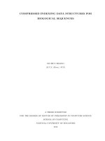
Figure 2.1: suffix tree of “cbcba”
2.2.1 Suffix tree and suffix array operations
Recall some definitions about suffix tree and suffix array from Section 1.2.4, let
A
S
and
T
S
denote the suffix array and suffix tree of string
S
, respectively. Any substring
x

of
S
can be represented by a pair of indexes (
st, ed
), called suffix range. The operation
lookup
(
i
) returns
A
S
[
i
]. Consider a suffix range (
st, ed
) in
A
S
for some string
P
[1
m
], the
operation backward-search(st, ed, c) returns another suffix range (st

, ed

) for cP [1 m].
For every node
u

in the suffix tree
T
S
, the string on the path from the root to
u
is
called the path label of the node u, denoted as label(u).
In this work, we require the following operations on the suffix tree:
• parent(u): return the parent node of node u.
• leaf-rank
(
u
): returns the number of leaves less than or equal to
u
in preorder
sequence.
• leaf-select(i): returns the leaf of the suffix tree which has rank i.
• leftmost-child(u): returns the leftmost child of the subtree rooted at u.
• rightmost-child(u): returns the rightmost child of the subtree rooted at u.
• lca(u, v): returns the lowest common ancestor of two leaves u and v.
• depth
(
u
): returns the depth of
u
. (i.e. the number of nodes from
u
to the root
minus one).
• level-ancestor(u, d): returns the ancestor of u with depth d.

• suffix-link
(
u
) returns a node
v
such that
label
(
v
) equals the string
label
(
u
) with
the first character removed.
13