Estimation based on pooled data in human biomonitoring and statistical genetics

ESTIMATION BASED ON POOLED DATA IN
HUMAN BIOMONITORING AND STATISTICAL
GENETICS
LI XIANG
(B.Sc., UNIVERSITY OF SCIENCE AND TECHNOLOGY OF CHINA)
A THESIS SUBMITTED
FOR THE DEGREE OF DOCTOR OF
PHILOSOPHY
DEPARTMENT OF STATISTICS AND APPLIED
PROBABILITY
NATIONAL UNIVERSITY OF SINGAPORE
2014
DECLARATION
I hereby declare that the thesis is my original
work and it has been written by me in its entirety.
I have duly acknowledged all the sources of
information which have been used in the thesis.
This thesis has also not been submitted for any
degree in any university previously.
Li Xiang
1
st
May 2014
ii
Thesis Supervisors
Anthony Kuk Yung Cheung Professor; Department of Statistics and
Applied Probability, National University of Singapore, Singapore,
117546, Singapore (Main)
Xu Jinfeng Assistant Professor; Division of Biostatistics, Department of
Population Health, New York University School of Medicine, New
York, NY 10016, USA (Co-supervisor)

iii
Papers and Manuscript
Kuk, A. Y., Li, X., and Xu, J. (2013a). A fast collapsed data method for
estimating haplotype frequencies from pooled genotype data with appli-
cations to the study of rare variants. Statistics in medicine , 32(8):1343–
1360.
Kuk, A. Y., Li, X., and Xu, J. (2013b). An em algorithm based on an
internal list for estimating haplotype distributions of rare variants from
pooled genotype data. BMC genetics, 14(1):1–17.
Li, X., Kuk, A. Y., and Xu, J. (2014). Empirical bayes gaussian likeli-
hood estimation of exposure distributions from pooled samples in human
biomonitoring. In second revision: Statistics in medicine.
iv
Acknowledgements
There are many people who have supported and guided me through the
journey. I would like to express my sincere gratitude and appreciation to
my supervisor, Professor Anthony Kuk for his unwavering support, con-
tinual guidance and many opportunities that broadened my experience in
Statistics. I would also like to thank my co-supervisor, Dr. Xu Jinfeng who
is very helpful and encouraging. I am thankful to Associate Professors Li
Jialiang and David Nott in my pre-qualifying exam committee for providing
critical insights and suggestions.
I want to take this opportunity to thank Associate Professor Zhang Jin-
Ting for his support in my PhD application. I am thankful to Professor Loh
Wei Liem for his kind advice and encouragement. I would like to express
special thanks to other faculty members and support staffs. I am grateful
to NUS for awarding me the Graduate Research Scholarship to pursue
research in my area of interest with financial independence.
I would also like to express my sincere thanks to my classmates and
friends, Tian Dechao, Huang Lei and Huang Zhipeng for their friendship

and encouragement in the journey. Finally, I am grateful to my family for
their moral support, especially my wife Wan Ling for her unconditional
love, support and encouragement without which this thesis would not have
been possible.
v
Contents
Declaration ii
Thesis Supervisors iii
Papers and Manuscript iv
Acknowledgements v
Summary ix
List of Tables x
List of Figures xiii
List of Abbreviations xv
1 Introduction 1
1.1 Human Biomonitoring . . . . . . . . . . . . . . . . . . . . . 2
1.1.1 Background . . . . . . . . . . . . . . . . . . . . . . . 2
1.1.2 Notation . . . . . . . . . . . . . . . . . . . . . . . . . 4
1.1.3 Existing methods . . . . . . . . . . . . . . . . . . . . 4
1.1.4 The focus of this topic . . . . . . . . . . . . . . . . . 8
1.2 Haplotype Frequency Estimation . . . . . . . . . . . . . . . 8
1.2.1 Background . . . . . . . . . . . . . . . . . . . . . . . 8
1.2.2 Notation . . . . . . . . . . . . . . . . . . . . . . . . . 10
1.2.3 Existing methods . . . . . . . . . . . . . . . . . . . . 11
1.2.4 The focus of this topic . . . . . . . . . . . . . . . . . 17
2 Human Biomonitoring 20
vi
Contents
2.1 Summary . . . . . . . . . . . . . . . . . . . . . . . . . . . . 21
2.2 Gaussian Estimation . . . . . . . . . . . . . . . . . . . . . . 23

2.3 First Analysis of the 2003-04 NHANES Data . . . . . . . . . 27
2.4 Empirical Bayes GLE . . . . . . . . . . . . . . . . . . . . . . 32
2.5 An Adaptive EB Estimator via Estimating the Mean-Variance
Relationship . . . . . . . . . . . . . . . . . . . . . . . . . . . 37
2.6 Further Analysis of the 2003-04 NHANES Data . . . . . . . 38
2.7 Bayesian Estimates . . . . . . . . . . . . . . . . . . . . . . . 46
2.8 Simulation Study . . . . . . . . . . . . . . . . . . . . . . . . 47
2.9 Discussion . . . . . . . . . . . . . . . . . . . . . . . . . . . . 58
3 Collapsed Data MLE 66
3.1 Summary . . . . . . . . . . . . . . . . . . . . . . . . . . . . 66
3.2 Statistical Models and Methods . . . . . . . . . . . . . . . . 69
3.2.1 Collapsed data estimator . . . . . . . . . . . . . . . . 69
3.2.2 Running time analysis and comparison with the EML
algorithm . . . . . . . . . . . . . . . . . . . . . . . . 74
3.2.3 Variance and efficiency formulae . . . . . . . . . . . . 83
3.3 An Analysis of Rare Variants Associated with Obesity . . . 88
3.4 Discussion and Extensions . . . . . . . . . . . . . . . . . . . 94
4 EM with an Internal List 99
4.1 Summary . . . . . . . . . . . . . . . . . . . . . . . . . . . . 99
4.2 Statistical Models and Methods . . . . . . . . . . . . . . . . 101
4.2.1 Collapsed data list . . . . . . . . . . . . . . . . . . . 101
4.2.2 EM with an internal list . . . . . . . . . . . . . . . . 102
4.3 Results . . . . . . . . . . . . . . . . . . . . . . . . . . . . . . 108
4.4 Discussion . . . . . . . . . . . . . . . . . . . . . . . . . . . . 121
5 Conclusions and Future Work 124
5.1 Conclusions . . . . . . . . . . . . . . . . . . . . . . . . . . . 124
5.1.1 Human biomonitoring . . . . . . . . . . . . . . . . . 124
5.1.2 Haplotype frequency estimation . . . . . . . . . . . . 125
5.2 Ongoing and Future Work . . . . . . . . . . . . . . . . . . . 127
5.2.1 Human biomonitoring . . . . . . . . . . . . . . . . . 127

5.2.2 Haplotype frequency estimation . . . . . . . . . . . . 130
vii
Contents
Bibliography 136
viii
Summary
Pooling is a cost-effective way to collect data. However, estimation is com-
plicated by the often intractable distributions of the observed pool averages.
In this thesis, we consider two applications involving pooled data. The first
is to use aggregate data collected from pools of individuals to estimate the
levels of individual exposure for various environmental biochemicals. We
propose a quasi empirical Bayes estimation approach based on a Gaussian
working likelihood which enables pooling of information across different de-
mographic groups. The new estimator out-performs an existing estimator
in simulation studies. We consider haplotype frequency estimation from
pooled genotype data in our second application. A quick collapsed data
estimator is proposed which does not lose much efficiency for rare genet-
ic variants. For more efficient estimates, we propose a way to construct a
data-based list of possible haplotypes to be used in conjunction with the
expectation maximization (EM) algorithm to make it more feasible compu-
tationally. For non-rare alleles, haplotype distributions cannot be estimated
well from pooled data, and a sensible strategy is to collect individual as
well as pooled genotype data. A calibration type estimator based on the
combined data is proposed which is more efficient than the estimator based
on individual data alone.
ix
List of Tables
2.1 Estimates of group-specific 95
th
percentiles using individ-

ual data based on nonparametric method and log-normal
assumption, and using pooled data based on Monte Car-
lo EM (MCEM) and Gaussian likelihood estimator (GLE),
with 95% confidence intervals in parentheses. . . . . . . . . . 30
2.2 Estimates of 95
th
percentiles using pooled data based on
group-specific Gaussian likelihood estimator (GLE), Caudil-
l’s estimator (Caudill), empirical Bayes Gaussian likelihood
estimator (EB-GLE) and EB-GLE with selected mean model
(EB-GLEM), with the 95% confidence intervals (CIs) con-
structed using three methods. . . . . . . . . . . . . . . . . . 40
2.3 Selection of log-linear model of mean exposure based on
pooled 2003-04 NHANES data by Gaussian AIC/BIC
∗
, and
parameter estimates under the selected model. . . . . . . . . 43
2.4 Mean, percent bias (% bias) and mean squared error (MSE)
of the group-specific Gaussian likelihood estimator (GLE),
empirical Bayes Gaussian likelihood estimator (EB-GLE)
and Caudills estimator of the 95
th
percentile P
95
for 24 de-
mographic groups based on 1000 simulations, together with
average length (L) and coverage (C) of the 95% confidence
intervals (CIs) based on three methods. . . . . . . . . . . . . 48
x
List of Tables

2.5 Mean, percent bias (% bias) and mean squared error (MSE)
of the empirical Bayes Gaussian likelihood estimator (EB-
GLE), adaptive empirical Bayes Gaussian likelihood estima-
tor (AEB-GLE) and empirical Bayes Gaussian likelihood es-
timator with selected mean model (EB-GLEM) of the 95
th
percentile P
95
for 24 demographic groups based on 1000 sim-
ulations, together with average length (L) and coverage (C)
of the 95% confidence intervals (CIs) based on three methods. 53
2.6 Mean, percent bias (% bias) and mean squared error (MSE)
of the Bayesian Gaussian likelihood estimator (B-GLE) un-
der various choices of the mixing distribution and B-GLE
under a selected mean model (B-GLEM) in estimating the
95
th
percentile P
95
for 24 demographic groups based on 1000
simulations, together with average length (L) and coverage
(C) of 95% credible intervals (CrIs). . . . . . . . . . . . . . . 56
2.7 Mean, percent bias (% bias) and mean squared error (MSE)
of the group-specific Gaussian likelihood estimator (GLE),
Caudills estimator, empirical Bayes Gaussian likelihood es-
timator (EB-GLE), adaptive empirical Bayes Gaussian like-
lihood estimator (AEB-GLE) and Bayesian Gaussian like-
lihood estimator (B-GLE) of the 95
th
percentile P

95
for 24
demographic groups of NHANES 2005-06 based on 1000 sim-
ulations, together with average length (L) and coverage (C)
of the 95% confidence intervals (CIs) based on three methods
and credible intervals (CrIs). . . . . . . . . . . . . . . . . . . 60
3.1 Running times in seconds of the collapsed data (CD) method
and the EML algorithm for estimating the haplotype distri-
butions of the 25 RVs in the MGLL region and the 32 RVs
in the FAAH region when 148 obese individuals are grouped
into pools of various sizes. . . . . . . . . . . . . . . . . . . . 77
3.2 Estimates of haplotype frequencies for the 25 RVs in the
MGLL region obtained from pooled genotype data of 148
obese individuals using the collapsed data (CD) method and
the EML algorithm, with standard errors in parentheses. . . 79
xi
List of Tables
3.3 Estimates of haplotype frequencies for the 32 RVs in the
FAAH region obtained from pooled genotype data of 148
obese individuals using the collapsed data (CD) method and
the EML algorithm, with standard errors in parentheses. . . 80
3.4 Estimates of haplotype frequencies and probabilities of vari-
ous variant combinations for the 25 RVs in the MGLL region
and the 32 RVs in the FAAH region obtained by collapsing
data from 148 cases and 150 controls, with k = 1 and stan-
dard errors in parentheses. . . . . . . . . . . . . . . . . . . . 92
3.5 Collapsed data estimates of haplotype frequencies for the 25
RVs in the MGLL region with and without “noise” added
to the pooled genotype data of 148 obese individuals, with
standard errors in parentheses. . . . . . . . . . . . . . . . . 96

4.1 Running times of EM algorithms based on different lists . . 104
4.2 Sufficient conditions for non-ancestral haplotype frequencies
to be increased by collapsing data . . . . . . . . . . . . . . . 106
4.3 Induced collapsed data frequencies . . . . . . . . . . . . . . 107
4.4 Haplotype frequency estimates in the MGLL region using
data from 148 obese individuals . . . . . . . . . . . . . . . . 110
4.5 Average estimates of haplotype frequencies for a 25 loci case 111
4.6 Average estimates of haplotype frequencies for a 32 loci case 113
xii
List of Figures
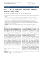
2.1 Plot of log (u
2
i
) versus log

¯
A
i

for the artificially pooled
NHANES 2003-04 data. The radius of the circle indicates
the relative weight of this data point in the weighted least
squares regression and the line represents the weighted least
squares fit. . . . . . . . . . . . . . . . . . . . . . . . . . . . . 39
3.1 Asymptotic relative efficiency of the collapsed data MLE
versus the complete data MLE of the haplotype frequency
of all zeros for various choices of the true frequency. . . . . . 85
4.1 Expected sum of squared errors of various haplotype fre-
quency estimators for a 25 loci case. Expected sum of squared
errors of various haplotype frequency estimators (EM-CDL:

EM with CD list; EM-ACDL: augmented CD list; EML: EM
with combinatorially determined list; CDMLE: collapsed da-
ta MLE; EM-TCDL: CD list with trimming and no augmen-
tation; EM-ATCDL: augmented and trimmed CD list; EM-
PL: EM with perfect list) based on 100 simulations of n pools
of k individuals each when the true haplotype distribution
over 25 loci is as given in Table 4.5. . . . . . . . . . . . . . 117
4.2 Expected sum of squared errors of various haplotype fre-
quency estimators for a 32 loci case. Expected sum of squared
errors of various haplotype frequency estimators (EM-CDL:
EM with CD list; EM-ACDL: augmented CD list; EML: EM
with combinatorially determined list; CDMLE: collapsed da-
ta MLE; EM-TCDL: CD list with trimming and no augmen-
tation; EM-ATCDL: augmented and trimmed CD list; EM-
PL: EM with perfect list) based on 100 simulations of n pools
of k individuals each when the true haplotype distribution
over 32 loci is as given in Table 4.6. . . . . . . . . . . . . . . 118
xiii
List of Figures
4.3 Expected sum of squared errors of the EM-ATCDL estimator
with fixed threshold (25 loci case). Expected sum of squared
errors of the EM-ATCDL estimator for various choices of
the threshold (Optimal threshold: the threshold obtained
by minimizing the averaged sum of squared errors; Average
adaptive threshold: adaptively chosen thresholds obtained
by minimizing the distance between
ˆ
f(0) and f(0) over the
grid 0.0001 to 0.002 in steps of 0.0001) based on 100 simula-
tions of n pools of k individuals each when the true haplotype

distribution over 25 loci is as given in Table 4.5. . . . . . . . 119
4.4 Expected sum of squared errors of the EM-ATCDL estimator
with fixed threshold (32 loci case). Expected sum of squared
errors of the EM-ATCDL estimator for various choices of
the threshold (Optimal threshold: the threshold obtained
by minimizing the averaged sum of squared errors; Average
adaptive threshold: adaptively chosen thresholds obtained
by minimizing the distance between
ˆ
f(0) and f(0) over the
grid 0.0001 to 0.002 in steps of 0.0001) based on 100 simula-
tions of n pools of k individuals each when the true haplotype
distribution over 32 loci is as given in Table 4.6. . . . . . . . 120
xiv
List of Abbreviations
AIC Akaike information criterion.
BIC Bayesian information criterion.
EM Expectation maximization.
GLE Gaussian likelihood estimator.
MCEM Monte Carlo expectation maximization.
MCMC Markov chain Monte Carlo.
MLE Maximum likelihood estimate.
xv
Chapter 1
Introduction
Pooling of samples is a cost effective and often efficient way to collect data.
The pooling design allows a large number of individuals from the popu-
lation to be sampled at reduced analytical costs. Estimation is, however,
complicated by the fact that the individual values within each pool are
not observed but are only known up to their average. In this thesis, we

consider two applications involving pooled data, i.e. human biomonitoring
and statistical genetics.
This chapter is organized as follows. Section 1.1 introduces the back-
ground of human biomonitoring (section 1.1.1), reviews the existing meth-
ods (section 1.1.3) and highlights the focus of this topic (section 1.1.4);
Section 1.2 briefly describes the haplotype frequency estimation (section
1.2.1), reviews some existing methods (section 1.2.3) and highlights the
focus of this topic (section 1.2.4).
1
Chapter 1. Introduction
1.1 Human Biomonitoring
1.1.1 Background
Human biomonitoring offers a way to better understand population expo-
sure to environmental chemicals by directly measuring the chemical com-
pounds or their metabolites in human specimens, such as blood and urine
(Sexton et al., 2004; Angerer et al., 2007). The early examples of biomon-
itoring could be traced back to the determination of lead in Kehoe et al.
(1933) or benzene metabolites in Yant et al. (1936), which were mainly
used to control the exposure to contaminants at the workplace. A more
recent example arose when blood and urine samples were taken from res-
cuers and examined for exposure to potentially toxic smoke from the rubble
after the World Trade Center collapse on 11 September 2001 (Erik, 2004).
Nowadays, more regular survey studies are conducted in various countries
or regions to determine a broad range of internal chemical concentrations
in general populations, like the National Health and Nutrition Examina-
tion Surveys (NHANES) in the U.S. and the German Environmental Survey
(GerES) in Germany. The data from biomonitoring are used to characterize
the concentration distributions of compounds among the general popula-
tion and to identify vulnerable groups with high exposure (Thornton et al.,
2002). Uncertainties in characterizing concentrations arise when exposure

measurements approach the limit of detection (LOD) or with insufficient
volume of material (Caudill, 2010; Caudill et al., 2007b). Despite continu-
ous improvement in analytical techniques, Caudill (2010) pointed out that
“the percentage of results below the LOD is not declining and may actu-
ally be increasing concurrently with decreasing exposure levels”. Another
2
1.1. Human Biomonitoring
problem in evaluating environmental exposures is the expense of measuring
some compounds as the cost generally increases with the accuracy of the
chemical assessment (Sexton et al., 2004). In the U.S., cost varies widely
from a few U.S. dollars for lead metals to thousands of U.S. dollars for diox-
ins and polychlorinated biphenyls (PCBs). When evaluating communities
or populations, the cost of biomonitoring can increase exponentially.
Pooling of samples can provide one possible solution to both problem-
s by yielding larger sample volumes and reducing the number of analytic
measurements to save cost (Bates et al., 2004, 2005; Caudill, 2011, 2012).
A weighted pooled sample design was first implemented in NHANES 2005-
06 (Caudill, 2012). The number of chemical measurements required was
reduced from 2201 to 228 and hence the study saved approximately $2.78
million at a cost of $1400 per testing. Estimation is, however, complicated
by the fact that the individual values within each pool are not observed
but are only known up to their average or weighted average. The distri-
bution of such averages is intractable when the individual measurements
are log-normally distributed, which is a common and realistic assumption
(Caudill, 2010). Furthermore, pooled samples may lose valuable informa-
tion on dispersion (Bignert et al., 1993) and lead to biased estimates of
central tendency (Caudill, 2011). Caudill et al. (2007a) proposed a method
to correct the bias of estimates obtained using pooled data from a log-
normal distribution. Caudill (2010) extended their method to characterize
the population distribution by using percentiles. More recently, Caudill

addressed estimation using information from an auxiliary source (Caudill,
2011) and extended the method to a weighted pooled sample design in a
special issue of Statistics in Medicine (Caudill, 2012). But Caudill’s esti-
3
Chapter 1. Introduction
mator is quite ad hoc, and its latest version (Caudill, 2012) relies on the
fitting of two straight lines with unexplained weights to perform some kind
of smoothing across demographic groups.
1.1.2 Notation
Suppose individual samples were grouped into n
i
pools of equal size K
in the i
th
demographic group, i = 1, · · · , d. Denote by X
ijk
the pollutant
concentration of individual k in the j
th
pool of the i
th
demographic group
with Y
ijk
= log X
ijk
∼ N (µ
i
, σ
2

i
) independently, where i = 1, · · · , d, j =
1, · · · , n
i
, k = 1, · · · , K. Assume the unweighed average A
ij
=

K
k=1
X
ijk
/K
is recorded for the j
th
pool in the i
th
group. All the methods using un-
weighed average can be easily extended to unequal weights ω
ijk
, A
ij,ω
=

K
k=1
ω
ijk
X
ijk

. The mean α
i
and variance β
2
i
of X
ijk
is given by
α
i
= E [X
ijk
] = exp

µ
i
+ σ
2
i
/2

, (1.1)
β
2
i
= var [X
ijk
] = exp

2µ

i
+ σ
2
i

exp

σ
2
i

− 1

= α
2
i

exp

σ
2
i

− 1

.
(1.2)
For the case of unweighed average, we can obtain the mean and variance
of A
ij

E [A
ij
] = E [X
ijk
] = α
i
, (1.3)
var [A
ij
] = var [X
ijk
] /K = β
2
i
/K. (1.4)
1.1.3 Existing methods
In this section, we briefly review the existing methods.
• Caudill et al. (2007a) noticed that the measured value of a pooled
4
1.1. Human Biomonitoring
sample A
ij
was an estimate of exp (µ
i
+ σ
2
i
/2), based on Equations (1.1)
and (1.3), but there was a positive bias when estimating µ
i

using log A
ij
alone. They proposed a way to correct this bias, which was equal to one-
half the variance of the logarithm of the individual samples constituting
the pool. The squared coefficient of variation (CV
2
i
) of A
ij
is given by
CV
2
i
=
var [A
ij
]
E [A
ij
]
2
=

exp

σ
2
i

− 1


/K. (1.5)
which could be used to calculate σ
2
i
after estimating CV
2
i
. The CV
2
i
can
be estimated as the ratio between sample variance and squared sample
mean of A
ij
for each demographic group. Due to the small number of pools
in some demographic groups, they estimated var [A
ij
] by using the range
based on var [A
ij
] = w
K
(A
i,max
− A
i,min
), where w
K
was the factor used

to convert an observed range for K samples to a variance estimate on
the basis of the distribution of the range of normally distributed samples
(Gosset, 1927), and A
i,max
and A
i,min
were the maximum and minimum
values in the i
th
demographic group respectively. Furthermore, they fit a
weighted least squares regression of CV
i
on the logarithm of the median in
the corresponding demographic group with weights n
2
i
. The fitted value

CV
i
was used to estimate σ
2
i
according to Equation (1.5). Then the estimate of
µ
i
was given by the average of the bias-corrected values
ˆµ
i
=


n
i
j=1
log A
ij
n
i
−
ˆσ
2
i
2
=

n
i
j=1
log A
ij
n
i
−
log

K

CV
2
i

+ 1

2
.
However, there is a lack of explanation for the use of weighted least squares
and its choice of weights.
• Caudill (2010) extended their method (Caudill et al., 2007a) to char-
5
Chapter 1. Introduction
acterize the population distribution by using percentiles and also provided
formulas of calculating confidence limits around the percentile estimate.
The p
th
percentile for log-normal populations was given by
P
i,p
= exp (µ
i
+ f
p
σ
∗
i
) (1.6)
where f
p
was the p
th
percentile of the standard normal distribution. Similar
method was used to estimate µ as described in Caudill et al. (2007a), ex-

cepting that in this paper he suggested using sample coefficient of variation
as a natural estimator instead (Caudill, 2010). He suggested several ways
to estimate σ
∗
i
in the Equation 1.6. One of them was to simply compute
the sample standard deviation of the bias-corrected values log A
ij
− ˆσ
2
i
/2.
Two-sided 100(1 − α)% confidence limits (LL
P
, UL
P
) around a percentile
estimate was computed by using a noncentral t distribution that can be
obtained from Table 1 of Odeh and Owen (1980).
• Caudill (2011) investigated ways to further reduce the bias in the
estimation by augmenting variance information from other studies. Simi-
lar technique was applied as in Caudill et al. (2007a), by using a weighted
least squares regression of CV
i
on the logarithm of the median in the corre-
sponding demographic group with weights n
2
i
. Augmentation can be made
by taking into account the data from other studies or other groups. They

found the increase in number of pools may help reduce the bias using the
same number of individuals, while the increase in the number of samples
in each pool may not.
• More recently, Caudill (2012) extended his own methods to a weighted
pooled sample design in a special issue of Statistics in Medicine. For sim-
plicity of the presentation, only the case of unweighed average is reviewed
6
1.1. Human Biomonitoring
here. In this paper, he slightly changed the assumption of the distribution
of individual measurement to Y
ijk
= log X
ijk
∼ N

µ
ij
, σ
2
ij

, with various
means and variances for each pool. The bias-corrected values changed to
log A
ij
− ˆσ
2
ij
/2, and hence the estimate of µ
i

was given by the average of
the bias-corrected values
ˆµ
i
=

n
i
j=1

log A
ij
− ˆσ
2
ij
/2

n
i
According to Equation 1.5, ˆσ
2
ij
= log

K

CV
2
ij
+ 1


.

CV
2
ij
was estimated
as the ratio between ˆσ
A
ij
and A
ij
, where ˆσ
A
ij
was the estimated standard
deviation of A
ij
. In order to obtain ˆσ
A
ij
, he fit a weighted least squares
regression of logarithm of ˆσ
A
i
on the logarithm of the median of A
ij
in
the corresponding demographic group with weights n
2

i
, and estimated ˆσ
A
ij
from the weighted least squares model by the corresponding pool measured
value A
ij
.
Equation (1.6) was used to estimate the percentile. He estimated σ
∗2
i
as the total (i.e. within-pool and among-pool) variance associated with
logarithm of the unmeasured individual samples. The within-pool com-
ponent of the variance was calculated as σ
2
i,within
=

n
i
j=1
ˆσ
2
ij
/n
i
and the
between-pool component as the sample variance of the bias-corrected val-
ues log A
ij

− ˆσ
2
ij
/2 in the demographic group. Furthermore, he fit another
weighted least squares regression of log (ˆσ
∗
i
) on ˆµ
i
with weights n
2
i
and
used the estimated ˆσ
∗∗
i
from the regression model as input to the percentile
estimate
ˆ
P
i,p
= exp (ˆµ
i
+ f
p
ˆσ
∗∗
i
).
7

Chapter 1. Introduction
1.1.4 The focus of this topic
Caudill proposed a few ways to characterize the concentration distributions
of compounds based on pooled samples (Caudill, 2010, 2011, 2012). How-
ever, Caudill’s estimator is quite ad hoc, and its latest version (Caudill,
2012) relies on the fitting of two straight lines with unexplained weights to
perform some kind of smoothing across demographic groups.
In chapter 2, we propose to replace the intractable distribution of the
pool averages by a Gaussian likelihood. An empirical Bayes Gaussian like-
lihood approach, as well as its Bayesian analogue, are developed to pool
information from various demographic groups by a mixed effect formula-
tion. Also discussed are methods to estimate the underlying mean-variance
relationship, and to select a good model for the means.
1.2 Haplotype Frequency Estimation
1.2.1 Background
In statistical genetics, the haplotype distribution is the joint distribution
of the allele types at, say, L loci. We will focus on bi-allelic loci in this
study so that each haplotype vector is a vector of binary values, and the
haplotype distribution is a multivariate binary distribution. The impor-
tance of haplotypes is well documented (Morris and Kaplan, 2002; Clark,
2004; Schaid, 2004) and reinforced more recently by the works of Muers
(2010) and Tewhey et al. (2011). By incorporating linkage disequilibrium
information from multiple loci, haplotype-based inference can lead to more
powerful tests of genetic association than single-locus analyses. Haplotype
distributions are usually estimated from individual genotype data which is
8
1.2. Haplotype Frequency Estimation
the sum of the maternal and paternal haplotype vectors of an individual.
As reviewed by Niu (2004) and Marchini et al. (2006), statistical approach-
es to haplotype inference based on individual genotype data are effective

and cost-efficient. These include the expectation-maximization (EM) type
algorithms for finding maximum likelihood estimates (MLE) (Excoffier and
Slatkin, 1995), and the Bayesian PHASE algorithm (Stephens and Scheet,
2005). Since DNA pooling is a popular and cost-effective way of collect-
ing data in genetic association studies (Sham et al., 2002; Norton et al.,
2004; Meaburn et al., 2006; Homer et al., 2008; Macgregor et al., 2008), the
EM algorithm and its variants have been extended by various authors (Ito
et al., 2003; Kirkpatrick et al., 2007; Zhang et al., 2008; Kuk et al., 2009)
to handle pooled genotype data (i.e., the sum of all K = 2k haplotype
vectors of all k individuals in a pool), whereas Pirinen et al. (2008), Gas-
barra et al. (2011) and Pirinen (2009) have extended Bayesian algorithms
using Markov Chain Monte Carlo (MCMC) or reversible jump MCMC
schemes. Also from a Bayesian perspective, Iliadis et al. (2012) conduct
deterministic tree-based sampling instead of MCMC sampling, but their
algorithm is feasible for small pool sizes only, even though the block size
can be arbitrary. Despite the falling costs of genotyping, the popularity
of the pooling strategy has not waned, with Kim et al. (2010) and Liang
et al. (2012) advocating the use of pooling for next-generation sequencing
data. The importance of pooling increases with the recent surge of inter-
est in rare variant analysis based on re-sequencing data (Mardis, 2008) to
explain missing heritability (Eichler et al., 2010) and diseases that cannot
be explained by common variants. Roach et al. (2011) predict that “haplo-
types that include rare alleles . . . will play an increasingly important role in
9
Chapter 1. Introduction
understanding biology, health, and disease”. Perhaps more so than in the
analysis of common variants, pooling has an important role to play in the
analysis of rare variants. This is because the standard methods for testing
genetic association are underpowered for rare variants due to insufficient
sample size as only a small percentage of study subjects would carry a rare

mutation, and pooling is a way to increase the chance of observing a rare
mutation. By using a pooling design, we could include more individuals in
a study at the same genotyping cost. The study by Kuk et al. (2010) shows
that pooling does not lead to much loss of estimation efficiency relative to
no pooling when the alleles are rare.
1.2.2 Notation
Focusing on bi-allelic loci, the two possible alleles at each locus can be
represented by “1” (the minor or variant allele) and “0” (the major allele).
As a result, the alleles at selected loci of a chromosome can be represented
by a binary haplotype vector. Since human chromosomes come in pairs,
there are 2 haplotype vectors for each individual, one maternal, and one
paternal. Suppose we have n pools of k individuals each so that there are
K = 2k haplotypes within each pool. Denote by Y
ij
= (Y
1ij
, · · · , Y
Lij
)

the
j
th
haplotype in the i
th
pool, where i = 1, · · · , n, j = 1, · · · , K, and L is
the number of loci to be genotyped. Assuming Hardy-Weinberg equilibrium,
the nK haplotype vectors are independent and identically distributed with
probability function
f(y

1
, · · · , y
L
) = P (Y
1ij
= y
1
, · · · , Y
Lij
= y
L
)
10