Temporally varying weight regression for speech recognition

Temporally Varying Weight
Regression for Speech Recognition
Shilin Liu
(B. Eng., Zhejiang University)
School of Computing
National University of Singapore
Dissertation submitted to the National University of Singapore
for the degree of Doctor of Philosophy
July 2014
Declaration
This dissertation is the result of my own work conducted at the School of
Computing, National University of Singapore. It does not include the out-
come of any work done in collaboration, except where stated. It has not been
submitted in whole or part for a degree at any other university.
To my best knowledge, the length of this thesis including footnotes and ap-
pendices is approximately 40,000 words.
Shilin Liu
Signature
Date
Acknowledgements
First of all, I would like to show my sincere gratitude to my advisor, Dr. SIM Khe
Chai, for his countless supervision, discussion and criticism throughout the work of this
dissertation. His guidance included from research suggestion, motivation, to scientific
writing. He has kept on arranging the weekly meeting up to four years to track my
research progress, and discuss challenging problems. 1 hour short weekly meeting has
inspired a lot of interesting works into this thesis. He was also providing the right balance
of supervision and freedom so that this thesis can be so manifold and fruitful. I would
also thank to many anonymous paper reviewers for the constructive comments, which
has significantly improved the quality of this thesis. Furthermore, this work could not
have been possible without many wonderful open source softwares: HTK toolkit from
the Machine Intelligence Laboratory at Cambridge University, Kaldi toolkit created by

researchers from Johns Hopkins University, Brno University of Technology and so on,
QuickNet from Speech Group in International Computer Science Institute at Berkeley.
I am also very thankful to the National University of Singapore for kindly providing 4
years research scholarship for my degree and many international conference travel grants.
I am also very grateful to Dr. SIM Khe Chai for kindly recruiting me as a research
assistant under the ARF funded project ”Haptic Voice Recognition: Perfecting Voice
Input with a Magic Touch”. I would also like to thank ISCA, IEEE SPS for providing
the conference travel grants.
I also owe my thanks to the members of Computational Linguistic lab led by Prof.
NG Hwee Tou. There are too many individuals to acknowledge, but I must thank, in no
particular order, WANG Guangsen, LI Bo, WANG Xuancong, WANG Xiaoxuan, WANG
Pidong, Lahiru Thilina Samarakoon, LU Wei. They have made the lab an interesting and
wonderful place to work in. I also learned a lot of other techniques, careers, experiences
from them. In addition, I must also thank my classmates and friends in Singapore,
FANG Shunkai, ZHANG Hanwang, FU Qiang, LU Peng, LI Feng, YI Yu, YU Jiangbo,
etc. They have organized many interesting and wonderful activities, which enriched my
life after working in Singapore.
Finally, I owe my biggest thank to my family in China for their endless support and
encouragement over the years. In particular, I would like to thank my girlfriend, LIU
Yilian who has always believed in me!
Contents
Table of Contents ix
List of Acronyms xii
List of Publications xiii
List of Tables xiii
List of Figures xiv
1 Introduction to Speech Recognition 1
1.1 Statistical Speech Recognition . . . . . . . . . . . . . . . . . . . . . . . . . 2
1.1.1 System Overview . . . . . . . . . . . . . . . . . . . . . . . . . . . . 2
1.1.2 Problem Formulation . . . . . . . . . . . . . . . . . . . . . . . . . . 3

1.1.3 Research Problems . . . . . . . . . . . . . . . . . . . . . . . . . . . 5
1.2 Thesis Organization . . . . . . . . . . . . . . . . . . . . . . . . . . . . . . . 6
2 Acoustic Modelling for Speech Recognition 8
2.1 Front-end Signal Processing and Feature Extraction . . . . . . . . . . . . . 8
2.2 Hidden Markov Model (HMM) for Acoustic modelling . . . . . . . . . . . . 14
2.2.1 HMM Formulation . . . . . . . . . . . . . . . . . . . . . . . . . . . 14
2.2.2 HMM Evaluation: Forward Recursion . . . . . . . . . . . . . . . . . 18
2.2.3 HMM Decoding: Viterbi Algorithm . . . . . . . . . . . . . . . . . . 19
2.2.4 HMM Estimation: Maximum Likelihood . . . . . . . . . . . . . . . 20
2.2.5 HMM Limitations . . . . . . . . . . . . . . . . . . . . . . . . . . . . 23
2.3 State-of-the-art Techniques . . . . . . . . . . . . . . . . . . . . . . . . . . . 24
2.3.1 Trajectory Modelling . . . . . . . . . . . . . . . . . . . . . . . . . . 24
2.3.1.1 Explicit Trajectory Modelling . . . . . . . . . . . . . . . . 25
2.3.1.2 Implicit Trajectory Modelling . . . . . . . . . . . . . . . . 27
2.3.2 Discriminative Training . . . . . . . . . . . . . . . . . . . . . . . . 29
2.3.3 Speaker Adaptation and Adaptive Training . . . . . . . . . . . . . . 31
iii
CONTENTS
2.3.3.1 Speaker Adaptation . . . . . . . . . . . . . . . . . . . . . 32
2.3.3.2 Speaker Adaptive Training . . . . . . . . . . . . . . . . . . 34
2.3.4 Noise Robust Speech Recognition . . . . . . . . . . . . . . . . . . . 35
2.3.4.1 Feature Enhancement . . . . . . . . . . . . . . . . . . . . 35
2.3.4.2 Model Compensation . . . . . . . . . . . . . . . . . . . . . 37
2.3.5 Deep Neural Network (DNN) . . . . . . . . . . . . . . . . . . . . . 40
2.3.5.1 Restricted Boltzmann Machine (RBM) . . . . . . . . . . . 41
2.3.5.2 DBN Pre-training . . . . . . . . . . . . . . . . . . . . . . 44
2.3.5.3 CD-DNN/HMM Fine-tuning and Decoding . . . . . . . . 44
2.3.5.4 Discussion . . . . . . . . . . . . . . . . . . . . . . . . . . . 46
2.3.6 Cross-lingual Speech Recognition . . . . . . . . . . . . . . . . . . . 46
2.3.6.1 Cross-lingual Phone Mapping . . . . . . . . . . . . . . . . 47

2.3.6.2 Cross-lingual Tandem features . . . . . . . . . . . . . . . . 48
2.4 Summary . . . . . . . . . . . . . . . . . . . . . . . . . . . . . . . . . . . . 49
3 Temporally Varying Weight Regression for Speech Recognition 51
3.1 Introduction . . . . . . . . . . . . . . . . . . . . . . . . . . . . . . . . . . . 52
3.2 Temporally Varying Weight Regression . . . . . . . . . . . . . . . . . . . . 53
3.3 Parameter Estimation . . . . . . . . . . . . . . . . . . . . . . . . . . . . . 56
3.3.1 Maximum Likelihood Training . . . . . . . . . . . . . . . . . . . . . 57
3.3.2 Discriminative Training . . . . . . . . . . . . . . . . . . . . . . . . 59
3.3.3 I-Smoothing . . . . . . . . . . . . . . . . . . . . . . . . . . . . . . . 61
3.4 Comparison to fMPE . . . . . . . . . . . . . . . . . . . . . . . . . . . . . . 61
3.5 Experimental Results . . . . . . . . . . . . . . . . . . . . . . . . . . . . . . 63
3.5.1 ML Training of TVWR . . . . . . . . . . . . . . . . . . . . . . . . . 64
3.5.2 MPE Training of TVWR . . . . . . . . . . . . . . . . . . . . . . . . 65
3.5.3 I-Smoothing for TVWR . . . . . . . . . . . . . . . . . . . . . . . . 68
3.5.4 Noisy Speech Recognition . . . . . . . . . . . . . . . . . . . . . . . 69
3.6 Summary . . . . . . . . . . . . . . . . . . . . . . . . . . . . . . . . . . . . 70
4 Multi-stream TVWR for Cross-lingual Speech Recognition 71
4.1 Introduction . . . . . . . . . . . . . . . . . . . . . . . . . . . . . . . . . . . 71
4.2 Multi-stream TVWR . . . . . . . . . . . . . . . . . . . . . . . . . . . . . . 72
4.2.1 Temporal Context Expansion . . . . . . . . . . . . . . . . . . . . . 73
4.2.2 Spatial Context Expansion . . . . . . . . . . . . . . . . . . . . . . . 75
4.2.3 Parameter Estimation . . . . . . . . . . . . . . . . . . . . . . . . . 75
4.3 State Clustering for Regression Parameters . . . . . . . . . . . . . . . . . . 76
4.3.1 Tree-based State Clustering . . . . . . . . . . . . . . . . . . . . . . 76
4.3.2 Implementation Details . . . . . . . . . . . . . . . . . . . . . . . . . 78
4.4 Experimental Results . . . . . . . . . . . . . . . . . . . . . . . . . . . . . . 78
iv
CONTENTS
4.4.1 Baseline Mono-lingual Recognition . . . . . . . . . . . . . . . . . . 79
4.4.2 Tandem Cross-lingual Recognition . . . . . . . . . . . . . . . . . . . 80

4.4.3 TVWR Cross-lingual Recognition . . . . . . . . . . . . . . . . . . . 80
4.5 Summary . . . . . . . . . . . . . . . . . . . . . . . . . . . . . . . . . . . . 83
5 TVWR: An approach to Combine the GMM and the DNN 84
5.1 Introduction . . . . . . . . . . . . . . . . . . . . . . . . . . . . . . . . . . . 84
5.2 Combining GMM and DNN . . . . . . . . . . . . . . . . . . . . . . . . . . 86
5.3 Regression of CD-DNN Posteriors . . . . . . . . . . . . . . . . . . . . . . . 88
5.4 Experimental Results . . . . . . . . . . . . . . . . . . . . . . . . . . . . . . 90
5.5 Summary . . . . . . . . . . . . . . . . . . . . . . . . . . . . . . . . . . . . 92
6 Adaptation and Adaptive Training for Robust TVWR 94
6.1 Robust TVWR using GMM based Posteriors . . . . . . . . . . . . . . . . . 95
6.1.1 Introduction . . . . . . . . . . . . . . . . . . . . . . . . . . . . . . . 95
6.1.2 Model Compensation for TVWR . . . . . . . . . . . . . . . . . . . 96
6.1.2.1 Acoustic Model Compensation . . . . . . . . . . . . . . . 97
6.1.2.2 Posterior Synthesizer Compensation . . . . . . . . . . . . 98
6.1.3 NAT Approximation using TVWR . . . . . . . . . . . . . . . . . . 99
6.1.4 Experimental Results . . . . . . . . . . . . . . . . . . . . . . . . . . 101
6.1.5 Summary . . . . . . . . . . . . . . . . . . . . . . . . . . . . . . . . 103
6.2 Robust TVWR using DNN based Posteriors . . . . . . . . . . . . . . . . . 104
6.2.1 Introduction . . . . . . . . . . . . . . . . . . . . . . . . . . . . . . . 104
6.2.2 Noise Adaptation and Adaptive Training . . . . . . . . . . . . . . . 106
6.2.2.1 Noise Model Estimation . . . . . . . . . . . . . . . . . . . 108
6.2.2.2 Canonical Model Estimation . . . . . . . . . . . . . . . . . 111
6.2.3 Joint Adaptation and Adaptive Training . . . . . . . . . . . . . . . 112
6.2.3.1 Speaker Transform Estimation . . . . . . . . . . . . . . . 114
6.2.3.2 Noise Model Estimation . . . . . . . . . . . . . . . . . . . 114
6.2.3.3 Canonical Model Estimation . . . . . . . . . . . . . . . . . 116
6.2.3.4 Training Algorithm . . . . . . . . . . . . . . . . . . . . . . 117
6.2.4 Experimental Results . . . . . . . . . . . . . . . . . . . . . . . . . . 118
6.2.5 Summary . . . . . . . . . . . . . . . . . . . . . . . . . . . . . . . . 121
7 Conclusions and Future Works 125

7.1 Conclusions . . . . . . . . . . . . . . . . . . . . . . . . . . . . . . . . . . . 125
7.2 Future Works . . . . . . . . . . . . . . . . . . . . . . . . . . . . . . . . . . 126
References 141
v
CONTENTS
A Appendix 142
A.1 Jacobian Issue . . . . . . . . . . . . . . . . . . . . . . . . . . . . . . . . . . 142
A.2 Constraint Derivation for TVWR . . . . . . . . . . . . . . . . . . . . . . . 143
A.3 Solver for Discriminative Training of TVWR . . . . . . . . . . . . . . . . . 144
A.4 Useful Matrix Derivatives . . . . . . . . . . . . . . . . . . . . . . . . . . . 146
vi
Summary
Automatic Speech Recognition (ASR) has been one of the most popular research areas
in computer science. Many state-of-the-art ASR systems still use the Hidden Markov
Model (HMM) for acoustic modelling due to its efficient training and decoding. HMM
state output probability of an observation is assumed to be independent of the other
states and the surrounding observations. Since temporal correlation between observations
exists due to the nature of speech, this assumption is poorly made for speech signal.
Although the use of the dynamic parameters and the Gaussian mixture models (GMM) has
greatly improved the system performance, implicitly or explicitly modelling the trajectory
temporal correlation can potentially improve the ASR systems.
Firstly, an implicit trajectory model called Temporally Varying Weight Regression
(TVWR) is proposed in this thesis. Motivated by the success of discriminative training of
time-varying mean (fMPE) or variance (pMPE), TVWR aims of modelling the temporal
correlation information using the temporally varying GMM weights. In this framework,
the time-varying information is represented by the compact phone/state posterior features
predicted from the long span acoustic features. The GMM weights are then temporally
adjusted through a linear regression of the posterior features. Both maximum likelihood
and discriminative training criteria are formulated for parameter estimation.
Secondly, TVWR is investigated for cross-lingual speech recognition. By leveraging

on the well-trained foreign recognizers, high quality posteriors can be easily incorporated
into TVWR to boost the ASR performance on low-resource languages. In order to take
advantages of multiple foreign resources, multi-stream TVWR is also proposed, where
multiple sets of posterior features are used to incorporate richer (temporal and spatial)
context information. Furthermore, a separate decision tree based state-clustering for the
TVWR regression parameters is used to better utilize the more reliable posterior features.
Third, TVWR is investigated as an approach to combine the GMM and the deep
neural network (DNN). As reported by various research groups, DNN has been found
to consistently outperform GMM and has become the new state-of-the-art for speech
recognition. However, many advanced adaptation techniques have been developed for
GMM based systems, while it is difficult to devise effective adaptation methods for DNNs.
This thesis proposes a novel method of combining the DNN and the GMM using the
TVWR framework to take advantage of the superior performance of the DNNs and the
robust adaptability of the GMMs. In particular, posterior grouping and sparse regression
are proposed to address the issue of incorporating the high dimensional DNN posterior
features.
Finally, adaptation and adaptive training of TVWR are investigated for robust speech
recognition. In practice, many speech variabilities exist, which will lead to poor recog-
nition performance for mismatched conditions. TVWR has not been formulated to be
vii
robust against those speech variabilities, such as background noises, transmission chan-
nels, speakers, etc. The robustness of TVWR can be improved by applying the adaptation
and adaptive training techniques, which have been developed for the GMMs. Adaptation
aims to change the model parameters to match the test condition using limited supervi-
sion data from either the reference or hypothesis. Adaptive training estimates a canonical
acoustic model by removing speech variabilities, such that adaptation can be more effec-
tive. Both techniques are investigated for the TVWR systems using either the GMM or
the DNN-based posterior features. Benchmark tests on the Aurora 4 corpus for robust
speech recognition showed that TVWR obtained 21.3% relative improvements over the
DNN baseline system and also outperformed the best system in the current literature.

Keywords: Temporally Varying Weight Regression, Trajectory Modelling, Acoustic
Modelling, Discriminative Training, Large Vocabulary Continuous Speech Recognition,
State Clustering, Sparse Regression, Adaptation, Adaptive Training
viii
List of Acronyms
ADC Analog-to-digital
AM Acoustic Model
ASR Automatic Speech Recognition
BM Baum Welch
BMM Buried Markov model
CD Context Dependent
CI Context Independent
cFDLR constrained Feature Discriminant Linear Regression
CMLLR Constrained Maximum Likelihood Linear Regression
CMN Cepstral Mean Normalization
CVN Cepstral Variance Normalization
CMVN Cepstral Mean&Variance Normalization
CNC Confusion Network Combination
CNN Convolutional Neural Network
DBN Deep Belief Network
DCT Discrete Cosine Transform
DFT Discrete Fourier Transform
DNN Deep Neural Network
DPMC Data-driven PMC
EM Expectation Maximization
FAHMM Factor Analyzed HMM
FFT Fast Fourier Transform
FMLLR Feature Maximum Likelihood Linear Regression
GMM Gaussian Mixture Model
GRBM Gaussian-Bernoulli RBM

HLDA Heteroscedastic Linear Discriminant Analysis
ix
HMM Hidden Markov Model
HTK HMM Toolkit
HTM Hidden Trajectory Model
KL Kullback-Leibler divergence
LDA Linear Discriminant Analysis
LM Language Model
LVCSR Large Vocabulary Continuous Speech Recognition
MAP Maximum a Posterior
MFCC Mel Frequency Cepstral Coefficients
ML Maximum Likelihood
MLLT Maximum Likelihood Linear Transform
MLE Maximum Likelihood estimation
MLP Multiple Layer Perceptron
MMI Maximum Mutual Information
MMSE Minimum Mean Square Error
MPE Minimum Phone Error
MLLR Maximum Likelihood Linear Regression
NAT Noise Adaptive Training
NN Neural Network
OOV Out-of-vocabulary
PER Phone Error Rate
PCA Principle Component Analysis
PLP Perceptual Linear Prediction Coefficients
PMC Parallel Model Combination
POS Part-of-speech
SVM Support Vector Machine
RBM Restricted Boltzmann Machine
RDLT Region Dependent Linear Transform

RNN Recurrent Neural Network
SAT Speaker Adaptive Training
SD Speaker Dependent
x
SI Speaker Independent
SER Sentence Error Rate
SLDS switching linear dynamical System
SNR Signal-to-noise Ratio
SSM Sstochastic Segment model
STC Semi-tied Covariance
STFT Short Time Fourier Transform
TPMC Trajectory-based PMC
TVWR Temporally Varying Weight Regression
VAD Voice Activity Detector
VTLN Vocal Tract Length Normalization
VTS Vector Taylor Series
WER Word Error Rate
WSJ Wall Street Journal
xi
List of Publications
1. Shilin Liu, Khe Chai Sim. “Joint Adaptation and Adaptive Training of TVWR
for Robust Automatic Speech Recognition,” accepted by Interspeech 2014
2. Shilin Liu, Khe Chai Sim. “On Combining DNN and GMM with Unsuper-
vised Speaker Adaptation for Robust Automatic Speech Recognition,” published
in ICASSP 2014
3. Shilin Liu, Khe Chai Sim. “Temporally Varying Weight Regression: a Semi-
parametric Trajectory Model for Automatic Speech Recognition,” published in
IEEE/ACM Transactions on Audio, Speech and Language Processing 2014
4. Shilin Liu, Khe Chai Sim. “Multi-stream Temporally Varying Weight Regression
for Cross-lingual Speech Recognition,” published in ASRU 2013

5. Shilin Liu, Khe Chai Sim. “An Investigation of Temporally Varying Weight Re-
gression for Noise Robust Speech Recognition,” published in Interspeech 2013
6. Shilin Liu, Khe Chai Sim. “Parameter Clustering for Temporally Varying Weight
Regression for Automatic Speech Recognition,” published in Interspeech 2013
7. Shilin Liu, Khe Chai Sim. “Implicit Trajectory Modelling Using Temporally Vary-
ing Weight Regression for Automatic Speech Recognition,” published in ICASSP
2012
8. Guangsen Wang, Bo Li, Shilin Liu, Xuancong Wang, Xiaoxuan Wang and Khe
Chai Sim. “Improving Mandarin Predictive Text Input By Augmenting Pinyin
Initials with Speech and Tonal Information,” published in ICMI 2012
9. Khe Chai Sim, Shilin Liu. “Semi-parametric Trajectory Modelling Using Tempo-
rally Varying Feature Mapping for Speech Recognition,” published in Interspeech
2010
xii
List of Tables
3.1 Comparison of 20k task performance for ML trained HMM and TVWR
systems. . . . . . . . . . . . . . . . . . . . . . . . . . . . . . . . . . . . . . 65
3.2 Different discriminatively trained system configuration descriptions. . . . . 66
3.3 Aurora 4 recognition results for various multi-condition trained systems. . . 69
4.1 WER(%) performance of HMM and TVWR fullset/subset baseline systems
for English and Malay speech recognition. . . . . . . . . . . . . . . . . . . . 79
4.2 WER(%) performance of various tandem systems with limited resources for
target English and Malay speech recognition. . . . . . . . . . . . . . . . . . 80
4.3 WER(%) performance of TVWR systems with or without context expansion
for target English and Malay speech recognition. . . . . . . . . . . . . . . . 81
4.4 WER(%) performance of various multi-stream TVWR systems with a sec-
ond state clustering and limited resources for target English and Malay
speech recognition. . . . . . . . . . . . . . . . . . . . . . . . . . . . . . . . . 82
5.1 WER(%) of various baseline systems with or without unsupervised speaker
adaptation. . . . . . . . . . . . . . . . . . . . . . . . . . . . . . . . . . . . 91

5.2 Comparison of the number of regression parameters per Gaussian compo-
nent and the WER (%) performance of various GMM+DNN/HMM systems
with or without context expansion and unsupervised speaker adaptation. . . 91
6.1 WER(%) for different approaches using clean training data. . . . . . . . . . 102
6.2 WER(%) for different approaches using multi-noise training data. . . . . . 103
6.3 Compact recognition results (WER%) of various baseline systems without
adaptation on Aurora4. . . . . . . . . . . . . . . . . . . . . . . . . . . . . . 120
6.4 Compact recognition results (WER%) of various systems on Aurora4 based
on adaptation and adaptive training. . . . . . . . . . . . . . . . . . . . . . 122
6.5 Full recognition results (WER%) of various baseline systems without adap-
tation on Aurora4. . . . . . . . . . . . . . . . . . . . . . . . . . . . . . . . 123
6.6 Complete recognition results (WER%) of various systems on Aurora4 based
on adaptation and adaptive training. . . . . . . . . . . . . . . . . . . . . . 124
xiii
List of Figures
1.1 Architecture of a typical speech recognition system. . . . . . . . . . . . . . 2
2.1 An example of waveform with 8 kHz sampling rate. . . . . . . . . . . . . . 9
2.2 An diagram of block processing waveform for feature extraction. . . . . . . 10
2.3 Spectrograms using different block size and the same 50% overlapping.
Middle: 40 ms block size(better frequency resolution); Bottom: 10 ms
block size(better time resolution). . . . . . . . . . . . . . . . . . . . . . . . 10
2.4 Mel filter banks with increasing widths, and Mel spectral coefficients. . . . 12
2.5 A left-to-right model topology of HMM for acoustic modelling . . . . . . . 15
2.6 A piece-wise stationary process in conventional HMM . . . . . . . . . . . . 16
2.7 A better trajectory representation of speech utterance . . . . . . . . . . . . 17
2.8 A typical model of the acoustical environment . . . . . . . . . . . . . . . . 38
2.9 A diagram of DBN pre-training process for DNN initialization, where square
box represents visible units while oval represents hidden units. . . . . . . . 41
2.10 A typical workflow to extract cross-lingual tandem features . . . . . . . . . 49
3.1 Comparison of MPE criterion for each discriminatively trained systems. . . 66

3.2 Comparison of 20k task for various discriminatively trained systems. . . . . 67
3.3 Iterative evaluation of TVWR.MPE1 with different I-Smoothing constant τ
R
. 68
4.1 A system diagram of multi-stream TVWR for cross lingual speech recognition. 74
4.2 A demonstration of disambiguating different phones with an additional de-
cision tree. . . . . . . . . . . . . . . . . . . . . . . . . . . . . . . . . . . . . 77
4.3 A summarized performance comparison of various systems using 1h English
training data. . . . . . . . . . . . . . . . . . . . . . . . . . . . . . . . . . . 82
4.4 A summarized performance comparison of various systems using 6h Malay
training data. . . . . . . . . . . . . . . . . . . . . . . . . . . . . . . . . . . 83
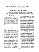
5.1 A schematic diagram showing the state output probability function of the
proposed GMM+DNN/HMM system. . . . . . . . . . . . . . . . . . . . . . 88
6.1 A diagram of joint adaptive training for TVWR. . . . . . . . . . . . . . . . 117
xiv
Chapter 1
Introduction to Speech Recognition
Speech is one of the most convenient communication approaches between humans and
machines. When the speech can be correctly recognized by the machine, it can offer many
conveniences for our daily life by avoiding tedious typing, for example, IBMs ViaVoice, a
desktop dictation system. After applying various natural language processing techniques
to analyze the semantic meaning of the recognized speech, many more useful applications
can be developed, such as speech translation, and automated call centers. In particular,
virtual personal assistant and its variants, such as iPhones Siri
1
, Google Now
2
, Bing
Search have become very popular recently in the mobile phones. These applications can
answer questions or execute commands by simply listening to the people.

The first technology behind these interesting applications is Automatic Speech Recog-
nition (ASR) system, which automatically converts a speech waveform to the word se-
quence or text. Although speech recognition has been studied since 1960s, it has not been
solved yet due to many practical challenges, such as speaker, environment, microphone
variabilities and so on. On the other hand, as speech varies in length, advanced classic
classifiers, such as Support Vector Machine (SVM) [1] and Neural Network (NN) [1] can-
not be directly applied for speech recognition. Hence, Hidden Markov Model (HMM) [2]
has become the most popular statistic acoustic model for the state-of-the-art ASR sys-
tems. Probability density function of the HMM state can be represented by a multivariate
Gaussian mixture model (GMM) [3]. A typical state-of-the-art context-dependent GMM-
HMM Large Vocabulary Continuous Speech Recognition (LVCSR) [4] system contains
tens of thousands of Gaussian components. Therefore, hundreds or thousands hours of
training data are needed for the robust estimation. Moreover, high system complexity
also increases the computing cost for both training and decoding. In practice, computer
clusters and cloud computing may be collaborated for providing recognition service for
mobile applications. In this chapter, a brief introduction of some essential components in
the ASR system will be presented.
1
/>2
/>1
1.1 Statistical Speech Recognition
1.1 Statistical Speech Recognition
In this section, speech recognition based on statistical method will be briefly introduced
from the system overview to the mathematical problem definition.
1.1.1 System Overview
Figure.1.1 shows a typical example of the ASR system, which consists of several impor-
tant components. ASR system takes a raw waveform file as input, and produces a most
likely transcription or text hidden in this file. The raw waveform file has to be passed
into the feature extraction component first. The purpose is to remove as much nui-
sance information as possible and keep manipulable and discriminable parameterization.

Hence, feature extraction is a process of leveraging the feature dimension and resolution.
For decades, researchers have engineered many acoustic features, such as Mel Frequency
Cepstral Coefficients (MFCC) and Perceptual Linear Prediction Coefficients (PLP). For
example, MFCC includes the short time-frequency analysis, filter bank analysis and dis-
crete cosine transform [5]. These coefficients are also referred to as the static parameters,
while their derivatives are usually calculated as the dynamic parameters. Concatenation
of these static and dynamic parameters becomes the final acoustic feature. Many other
advanced techniques also exist for post-processing of these fundamental acoustic features,
such as Linear Discriminant Analysis (LDA) [6], Heteroscedastic LDA (HLDA) [7], Mul-
tiple Layer Perceptron (MLP) [8] and so on. More details about the feature extraction
will be given in the next chapter.
Feature
Extraction
Lexicon
Models
Language
Models
Speech
Recognition
Post
Processing
Acoustic
Models
This is an
example.
Input waveform
Output Text
Figure 1.1: Architecture of a typical speech recognition system.
The speech recognition component includes three essential sub-components:
2

1.1 Statistical Speech Recognition
Acoustic Modelling
Acoustic model aims to discriminate different sound unit (such as phoneme, sylla-
ble or word) given the observation. Statistic acoustic model is usually employed
to learning their characteristics due to existing many speech variabilities. In addi-
tion, large amount of speech data with the correct transcription are also needed for
supervised training.
Language Modelling
Statistical language model is usually used to calculate the prior probability of a word
sequence. It has been widely used in many other areas, such as information retrieval,
part-of-speech tagging, etc. In speech recognition, it is primarily used to build the
searching network weighted by word transition probability. As the language model
complexity grows exponentially with respect to its dependency order, lower order
language model is usually applied for full decoding while higher order language
model is used for re-scoring.
Lexical Modelling
Lexical model is the connection between acoustic and language models. It is particu-
larly important when the acoustic model is based on the phoneme level, which is the
usual case. Lexical model builds the mapping between word and its pronunciation:
a phone sequence. If a word has multiple pronunciations, pronunciation probabili-
ties may be modelled for a better recognition. During recognition, vocabulary size is
always limited, which can lead to failure of recognition for those out-of-vocabulary
(OOV) words.
The post processing component is usually referred to as the system evaluation. In this
thesis, I will pay more specific attention on the recognition accuracy, which can be mea-
sured by the difference between the recognized hypothesis and the reference. Depending
on the purpose of evaluation, different error/distance metrics can be applied: Sentence
Error Rate (SER), Word Error Rate (WER), Phone Error Rate (PER). As an utterance
can be represented as a sequence of tokens (words or phones), Levenshtein distance has
been widely used to calculate WER and PER.

1.1.2 Problem Formulation
Due to the nature of speech recognition, it can be viewed as finding the hidden word se-
quence of an incoming speech utterance. Mathematically, this problem can be formulated
as searching a most likely word sequence given the speech utterance:
ˆ
W
N
1
= arg max
W
N
1
P (W
N
1
|O
T
1
, θ) (1.1)
3
1.1 Statistical Speech Recognition
where W
N
1
is a N-words sequence, O
T
1
is a T -frames observation sequence representing the
given utterance, θ are the underlying model parameters. One biggest challenge here is
that N is unknown during recognition. Assuming that the vocabulary size is V , the search

space would be V
N
. In other words, the ASR system may be infeasible if the recognition
algorithm is not carefully designed. Two categories of approaches may be applied to solve
this problem [1]:
Probabilistic Generative Model
This approach aims to model the class-conditional densities P(O
T
1
|W
N
1
), as well as
the class priors P (W
N
1
), which can be then used to compute the posterior probabil-
ities p(W
N
1
|O
T
1
) through the Bayes’ theorem. A typical example is Hidden Markov
Model (HMM) [9].
Probabilistic Discriminative Model
This approach directly computes the posterior probability of the class W
N
1
with-

out modelling class-conditional densities. One example for speech recognition is
Conditional Random Field [10].
In the case of using the generative model, according to the Bayes’ theorem, the con-
ditional probability can be rewritten as:
ˆ
W
N
1
= arg max
W
N
1
P (O
T
1
|W
N
1
, θ
AM
)P (W
N
1
|θ
LM
)
P (O
T
1
|θ)

∝ arg max
W
N
1
P (O
T
1
|W
N
1
, θ
AM
)P (W
N
1
|θ
LM
) (1.2)
where θ
AM
and θ
LM
are the acoustic model and language model parameters, respectively.
Since both N and the alignment between the observation and word sequence are unknown,
many famous probabilistic classifiers, such as SVM, NN cannot be applied directly. The
ability of modelling varying length of the speech makes the Hidden Markov Model (HMM)
as the most popular acoustic model. P (O
T
1
|W

N
1
, θ
AM
) is also called acoustic model score,
which depends on the underlying acoustic model. For instance, if the HMM is applied for
acoustic modelling, it will contain the state emission and transition probabilities.
Regarding the language model score, P(W
N
1
|θ
LM
), further factorization can be per-
formed such as:
P (W
N
1
|θ
LM
) = P (w
1
|θ
LM
)
N

i=2
P (w
i
|W

i−1
1
, θ
LM
) (1.3)
where w
i
is the i-th word of the word sequence, while W
i−1
1
is a word sequence occurring
before word w
i
. In practice, it is difficult to compute P (w
i
|W
i−1
1
, θ
LM
) for each i, which
requires a lot of training examples and memories. Therefore, approximation is made to
obtain a more tractable language model such that
P (w
i
|W
i−1
1
, θ
LM

) ≈ P(w
i
|w
i−1
, w
i−2
, w
i−n+1
, θ
LM
) (1.4)
4
1.1 Statistical Speech Recognition
where n defines the order of dependence on its preceding words, a.k.a. n-gram language
model. The typical way to utilize the language model for speech recognition is to use
lower order language model to build a smaller search network, generate hypotheses, and
then use higher order language model to re-calculate the language model score.
So far, the discussion has assumed that the acoustic and language models are given.
Hence, the remaining problem is how to perform training and decoding. Training is to
search optimal parameters for θ
AM
, θ
LM
such that the correct word sequence can have
the highest probability given the speech. Supervision based parameter training has to
be performed due to the nature of the speech recognition. In addition, training criteria
should be carefully chosen by leveraging the training efficiency and recognition accuracy.
Decoding is to search the most likely word sequence based on both acoustic and language
model scores. As the number of all possible word sequences could be numerically infinite,
decoding usually works together with various pruning strategies, such as the beam-search.

In summary, statistical speech recognition includes many essential components, and
each of them can have serious impact on the final system performance. To my best
knowledge, global optimal solution has not been found for each component yet, therefore
there are still many open research topics for each component. In this thesis, the focus
will be on acoustic modelling.
1.1.3 Research Problems
Speech recognition research has been going on since the 1960s, but it has not been com-
pletely solved yet. This is due to existing many speech related variations during the
speech recognition:
• temporal and spatial variations in speech signals (e.g. duration, trajectory)
• inter-speaker variations (e.g. gender, age, non-native speakers)
• intra-speaker variations (e.g. physical body condition)
• channel variations (e.g. microphone, background noise, bandwidths)
• difficulties in modelling syntax and semantics of languages (e.g. words with different
part-of-speech (POS) or meanings but with the same pronunciation)
• difficulties in modelling domain information (e.g. literature, finance, science, tele-
phone)
• limited resources for some languages (e.g. limited transcribed training data)
5
1.2 Thesis Organization
In practice, it is difficult to estimate a speech recognition system to deal with all possible
variations. Many applications based on ASR technology work well only on some working
conditions. For example, Siri on the iPhone does not work well for non-native English
speakers or in a noisy environment. In this thesis, I will focus on dealing with part
of above research problems, such as trajectory modelling, speaker variations, channel
variations and limited resources issues.
1.2 Thesis Organization
In chapter 2, the most widely used acoustic model, Hidden Markov Models (HMM) will be
introduced. First, front-end signal processing for feature extraction is introduced. Next,
technical details about formulation, parameter estimation and decoding for GMM-HMM

system are discussed. Finally, limitations of HMM are discussed and various advanced
techniques are reviewed for solving these limitations, including trajectory modelling, dis-
criminative training, adaptation and adaptive training, deep neural network (DNN) and
cross-lingual speech recognition.
In chapter 3, temporally varying weight regression (TVWR) [11, 12] framework is
proposed as a new semi-parametric trajectory model for speech recognition. First, a formal
probabilistic formulation is given. Next, parameter estimations using both maximum
likelihood and discriminative training criteria are introduced. In addition, I-Smoothing
is also proposed as an interpolation of two training criteria for a better generalization.
Last, experiments are conducted to evaluate the performance based on different training
criteria and corpora.
In chapter 4, TVWR [13] is investigated for cross-lingual speech recognition. In partic-
ular, temporal and spatial context expansions are proposed to incorporate richer context
information for a better recognition accuracy. In addition, a second tree-based state
clustering is also proposed for the regression parameters. Experiments are conducted to
evaluate this method for cross-lingual speech recognition.
In chapter 5, TVWR is investigated as an approach to combine two state-of-the-arts:
GMM and DNN. The goal is to take advantage of the advanced adaptation techniques
from GMM and the superior recognition accuracy from DNN. In order to handle the
high system complexity of incorporating the high dimensional DNN posteriors, posterior
grouping and sparse regression are proposed. Experiments are conducted to evaluate
unsupervised speaker adaptation for TVWR using DNN posteriors.
In chapter 6, adaptation and adaptive training are studied for robust TVWR. Adapta-
tion and adaptive training have been widely used to improve the robustness of the speech
recognition system. Depending on the types of posteriors features, robust TVWR is inves-
tigated via two directions: GMM based posteriors, DNN based posteriors. If GMM based
posteriors are used, model compensation can be performed for both the acoustic model
and the posterior synthesizer. This approach is also investigated as an approximation of
6
1.2 Thesis Organization

noise adaptive training. On the other hand, as DNN has been found outperforming GMM
for various speech recognition tasks, using DNN posteriors can significantly boost the per-
formance of the TVWR system. Furthermore, joint adaptation and adaptive training of
TVWR using DNN based posteriors are investigated.
In chapter 7, the conclusion is drawn and some future works are discussed.
7
Chapter 2
Acoustic Modelling for Speech
Recognition
Hidden Markov Model (HMM) [2] has been widely used as acoustic model for automatic
speech recognition for decades. As HMM can subsume the speech data with varying
duration, it can be adopted as a generative model to synthesize speech. Due to its
probabilistic nature, HMM can also be used as a statistical classifier to perform the speech
recognition. After incorporating the Gaussian mixture model (GMM) [3] as the state
probability density function, efficient training and decoding algorithms can be derived for
GMM/HMM. In this chapter, the attention will be paid on a GMM/HMM recognition
system and the advanced state-of-the-art techniques. The important components contain
front-end signal processing and parameterization, system evaluation, Viterbi decoding and
parameter estimation. Popular state-of-the-art techniques will cover trajectory modelling,
discriminative training, adaptation and speaker adaptive training, deep neural networks,
cross-lingual speech recognition. Finally, limitations of the current GMM/HMM system
and some possible works to circumvent those issues will be discussed.
2.1 Front-end Signal Processing and Feature Extrac-
tion
Typically, speech is stored in the waveform file format. Speech recording contains a
analog-to-digital conversion (ADC): converting the analog voltage variations caused by
air pressure to digital sound. Two key concepts are happening in this process: sampling
and quantization, which also serve as the measure of sound quality. When people speak to
the microphone, the air pressure is recorded according to a fixed time interval. If a speech
waveform is sampled at 16000 times per second, it will have a sampling rate of 16 kHz (kilo

Hertz). Higher sampling rate can lead to a better sound quality, but also requires more
8
2.1 Front-end Signal Processing and Feature Extraction
storages. Quantization is used to convert the sampled continuous waveform amplitudes
to discrete values. Depending on how many bits will be used for the quantization, the
accuracy of such approximation will be different. In usual, 8 bits and 16 bits will be used
to represent a total of 256 and 65536 possible quantization levels respectively.
2.6 2.7 2.8 2.9 3 3.1 3.2 3.3 3.4 3.5
−0.08
−0.06
−0.04
−0.02
0
0.02
0.04
0.06
Time (in seconds)
Amplitude
Figure 2.1: An example of waveform with 8 kHz sampling rate.
As the speech waveform contains too much speech-unrelated information, spectral
analysis is usually applied, such as Discrete Fourier Transform (DFT) or fast Fourier
Transform (FFT). Modern speech parameterization usually employs block processing
as shown in Figure. 2.2, which assumes that a short block/frame of samples are quasi-
stationary. Frame size is a compromise between the accuracy of time-frequency analysis
(needs more samples) and the validness of quasi-stationary assumption (needs fewer sam-
ples). Frame shiftting is another factor during block processing, which is used to capture
the dynamics of speech. These two factors determine the final number of frames given a
speech utterance.
The purpose of block processing is to find a good representation of speech signal, which
can be then used to distinguish different speech patterns. As speech pattern is composed

of time and frequency, compromise between these two resolutions needs to be made. In
order to better understand this concept, spectrogram is introduced. Spectrogram is a
two-dimensional visual representation of the Short Time Fourier Transform (STFT) of a
time signal. As shown in Figure. 2.3, the spectrogram using 40 ms block size shows better
frequency resolution as more samples can be used to calculate more accurate frequencies.
However, when compared to the bottom figure using 10 ms block size, the middle one
clearly shows worse resolution in the time domain. Except that, there are still many
other techniques used during spectral analysis, such as windowing (used for smoothing
the edge of block processing), pre-emphasis. Pre-emphasis is used to improve the overall
9
2.1 Front-end Signal Processing and Feature Extraction
Window Duration
Frame Period
Block n
Block n+1
…etc
feature n feature n+1
Figure 2.2: An diagram of block processing waveform for feature extraction.
Figure 2.3: Spectrograms using different block size and the same 50% overlapping. Middle:
40 ms block size(better frequency resolution); Bottom: 10 ms block size(better time
resolution).
10