Robust low dimensional structure learning for big data and its applications

Robust low-dimensional structure learning
for big data and its applications
JIASHI FENG
(B.Eng., USTC)
A THESIS SUBMITTED FOR
THE DEGREE OF DOCTOR OF PHILOSOPHY
DEPARTMENT OF ELECTRICAL AND COMPUTER ENGINEERING
NATIONAL UNIVERSITY OF SINGAPORE
2014
Declaration
I hereby declare that this thesis is my original work and it has been written by me
in its entirety.
I have duly acknowledged all the sources of information which have been used
in the thesis.
This thesis has also not been submitted for any degree in any university previ-
ously.
Jiashi Feng
May 23, 2014
1
Acknowledgements
First and foremost, I am deeply indebted to my two advisors, Professor Shuicheng
Yan and Professor Huan Xu. It has been an honor to be Ph.D. student co-advised
by them. Their support and advice have been invaluable for me, in terms of both
personal interaction and professionalism. I have benefited from their broad range
of knowledge, deep insight and thorough technical guidance in each and every step
of my research during the last four years. I thoroughly enjoyed working with them.
Without their inspiration and supervision, this thesis would never have happened.
I am very grateful to Professor Trevor Darrell of the University of California at
Berkeley for providing me with the opportunity of visiting his group at Berkeley.
I was impressed by his enthusiasm and curiosity, and there I met many great re-
searchers. I am fortunate to have had the chance to collaborate with Professor Shie

Mannor at Technion, an experience that helped produce a significant portion of this
thesis.
I would thank my friends at LV group, Qiang Chen, Zheng Song, Mengdi Xu,
Jian Dong, Wei Xia, Tam Nguyen, Luoqi Liu, Junshi Huang, Min Lin, Canyi Lu,
and others. They have created a very pleasant atmosphere in which to conduct
research and live my life. I am very grateful to my senior Bingbing Ni for helping
me at the beginning of my PhD career. Special thanks goes to Si Liu, Hairong Liu,
Professor Congyan Lang and Professor Zilei Wang. The time we work together is
my most precious moment in Singapore.
Finally, thanks to my parents for their love and support.
2
Contents
1 Introduction 15
1.1 Background and Related works . . . . . . . . . . . . . . . . . . . . . 16
1.1.1 Low-dimensional Structure Learning . . . . . . . . . . . . . . 16
1.1.2 Robustness in Structure Learning . . . . . . . . . . . . . . . . 17
1.1.3 Online Learning . . . . . . . . . . . . . . . . . . . . . . . . . 18
1.2 Thesis Focus and Main Contributions . . . . . . . . . . . . . . . . . 19
1.3 Structure of The Thesis . . . . . . . . . . . . . . . . . . . . . . . . . 22
2 Robust PCA in High-dimension: A Deterministic Approach 23
2.1 Introduction . . . . . . . . . . . . . . . . . . . . . . . . . . . . . . . . 23
2.2 Related Work . . . . . . . . . . . . . . . . . . . . . . . . . . . . . . . 25
2.3 The Algorithm . . . . . . . . . . . . . . . . . . . . . . . . . . . . . . 27
2.3.1 Problem Setup . . . . . . . . . . . . . . . . . . . . . . . . . . 27
2.3.2 Deterministic HR-PCA Algorithm . . . . . . . . . . . . . . . 28
2.4 Simulations . . . . . . . . . . . . . . . . . . . . . . . . . . . . . . . . 32
2.5 Proof of Theorem 1 . . . . . . . . . . . . . . . . . . . . . . . . . . . . 34
2.5.1 Validity of the Robust Variance Estimator . . . . . . . . . . . 35
2.5.2 Finite Steps for a Good Solution . . . . . . . . . . . . . . . . 38
2.5.3 Bounds on the Solution Performance . . . . . . . . . . . . . . 40

2.6 Proof of Corollary 1 . . . . . . . . . . . . . . . . . . . . . . . . . . . 43
2.7 Proof of Theorem 5 . . . . . . . . . . . . . . . . . . . . . . . . . . . . 46
2.8 Proof of Theorem 7 . . . . . . . . . . . . . . . . . . . . . . . . . . . . 47
3
2.9 Chapter Summary . . . . . . . . . . . . . . . . . . . . . . . . . . . . 51
3 Online PCA for Contaminated Data 52
3.1 Introduction . . . . . . . . . . . . . . . . . . . . . . . . . . . . . . . . 52
3.2 Related Work . . . . . . . . . . . . . . . . . . . . . . . . . . . . . . . 54
3.3 The Algorithm . . . . . . . . . . . . . . . . . . . . . . . . . . . . . . 55
3.3.1 Problem Setup . . . . . . . . . . . . . . . . . . . . . . . . . . 55
3.3.2 Online Robust PCA Algorithm . . . . . . . . . . . . . . . . . 57
3.4 Main Results . . . . . . . . . . . . . . . . . . . . . . . . . . . . . . . 58
3.5 Proof of The Results . . . . . . . . . . . . . . . . . . . . . . . . . . . 61
3.6 Simulations . . . . . . . . . . . . . . . . . . . . . . . . . . . . . . . . 64
3.7 Technical Lemmas . . . . . . . . . . . . . . . . . . . . . . . . . . . . 66
3.8 Proof of Lemma 6 . . . . . . . . . . . . . . . . . . . . . . . . . . . . 67
3.9 Proof of Lemma 7 . . . . . . . . . . . . . . . . . . . . . . . . . . . . 68
3.10 Proof of Lemma 8 . . . . . . . . . . . . . . . . . . . . . . . . . . . . 69
3.11 Proof of Lemma 9 . . . . . . . . . . . . . . . . . . . . . . . . . . . . 70
3.12 Proof of Theorem 10 . . . . . . . . . . . . . . . . . . . . . . . . . . . 71
3.13 Chapter Summary . . . . . . . . . . . . . . . . . . . . . . . . . . . . 75
4 Online Optimization for Robust PCA 77
4.1 Introduction . . . . . . . . . . . . . . . . . . . . . . . . . . . . . . . . 77
4.2 Related Work . . . . . . . . . . . . . . . . . . . . . . . . . . . . . . . 79
4.3 Problem Formulation . . . . . . . . . . . . . . . . . . . . . . . . . . . 80
4.3.1 Notation . . . . . . . . . . . . . . . . . . . . . . . . . . . . . . 80
4.3.2 Objective Function Formulation . . . . . . . . . . . . . . . . 81
4.4 Stochastic Optimization Algorithm for OR-PCA . . . . . . . . . . . 83
4.5 Algorithm solving Problem (4.7) . . . . . . . . . . . . . . . . . . . . 85
4.6 Proof Sketch . . . . . . . . . . . . . . . . . . . . . . . . . . . . . . . 86

4.7 Proof of Lemma 12 . . . . . . . . . . . . . . . . . . . . . . . . . . . . 88
4.8 Proof of Lemma 13 . . . . . . . . . . . . . . . . . . . . . . . . . . . . 90
4.9 Proof of Theorem 12 . . . . . . . . . . . . . . . . . . . . . . . . . . . 93
4
4.10 Proof of Theorem 13 . . . . . . . . . . . . . . . . . . . . . . . . . . . 95
4.11 Proof of Theorem 14 . . . . . . . . . . . . . . . . . . . . . . . . . . . 96
4.12 Proof of Theorem 15 . . . . . . . . . . . . . . . . . . . . . . . . . . . 98
4.13 Proof of Theorem 16 . . . . . . . . . . . . . . . . . . . . . . . . . . . 99
4.14 Technical Lemmas . . . . . . . . . . . . . . . . . . . . . . . . . . . . 101
4.15 Simulations . . . . . . . . . . . . . . . . . . . . . . . . . . . . . . . . 103
4.15.1 Medium-scale Robust PCA . . . . . . . . . . . . . . . . . . . 103
4.15.2 Large-scale Robust PCA . . . . . . . . . . . . . . . . . . . . . 106
4.15.3 Robust Subspace Tracking . . . . . . . . . . . . . . . . . . . . 107
4.16 Chapter Summary . . . . . . . . . . . . . . . . . . . . . . . . . . . . 110
5 Geometric 
p
-norm Feature Pooling for Image Classification 111
5.1 Introduction . . . . . . . . . . . . . . . . . . . . . . . . . . . . . . . . 111
5.2 Related Work . . . . . . . . . . . . . . . . . . . . . . . . . . . . . . . 114
5.3 Geometric 
p
-norm Feature Pooling . . . . . . . . . . . . . . . . . . . 115
5.3.1 Pooling Methods Revisit . . . . . . . . . . . . . . . . . . . . . 116
5.3.2 Geometric 
p
-norm Pooling . . . . . . . . . . . . . . . . . . . 117
5.3.3 Image Classification Procedure . . . . . . . . . . . . . . . . . 118
5.4 Towards Optimal Geometric Pooling . . . . . . . . . . . . . . . . . . 119
5.4.1 Class Separability . . . . . . . . . . . . . . . . . . . . . . . . 119
5.4.2 Spatial Correlation of Local Features . . . . . . . . . . . . . . 119

5.4.3 Optimal Geometric Pooling . . . . . . . . . . . . . . . . . . . 121
5.5 Experiments . . . . . . . . . . . . . . . . . . . . . . . . . . . . . . . . 122
5.5.1 Effectiveness of Feature Spatial Distribution . . . . . . . . . . 123
5.5.2 Object and Scene Classification . . . . . . . . . . . . . . . . . 124
5.6 Chapter Summary . . . . . . . . . . . . . . . . . . . . . . . . . . . . 128
6 Auto-grouped Sparse Representation for Visual Analysis 130
6.1 Introduction . . . . . . . . . . . . . . . . . . . . . . . . . . . . . . . . 130
6.2 Related Work . . . . . . . . . . . . . . . . . . . . . . . . . . . . . . . 133
6.3 Problem Formulation . . . . . . . . . . . . . . . . . . . . . . . . . . . 134
5
6.4 Optimization Procedure . . . . . . . . . . . . . . . . . . . . . . . . . 136
6.4.1 Smooth Approximation . . . . . . . . . . . . . . . . . . . . . 136
6.4.2 Optimization of the Smoothed Objective Function . . . . . . 137
6.4.3 Convergence Analysis . . . . . . . . . . . . . . . . . . . . . . 137
6.4.4 Complexity Discussions . . . . . . . . . . . . . . . . . . . . . 138
6.5 Experiments . . . . . . . . . . . . . . . . . . . . . . . . . . . . . . . . 139
6.5.1 Toy Problem: Sparse Mixture Regression . . . . . . . . . . . 139
6.5.2 Multi-edge Graph For Image Classification . . . . . . . . . . 140
6.5.3 Motion Segmentation . . . . . . . . . . . . . . . . . . . . . . 144
6.6 Chapter Summary . . . . . . . . . . . . . . . . . . . . . . . . . . . . 146
7 Conclusions 148
7.1 Summary of Contributions . . . . . . . . . . . . . . . . . . . . . . . . 148
7.2 Open Problems and Future research . . . . . . . . . . . . . . . . . . 150
6
Summary
The explosive growth of data in the era of big data has presented great challenges to
traditional machine learning techniques, since most of them are difficult to apply for
handling large-scale, high-dimensional and dynamically changing data. Moreover,
most of the current low-dimensional structure learning methods are fragile to the
noise explosion in high-dimensional regime, data contamination and outliers, which

however are ubiquitous in realistic data. In this thesis, we propose deterministic
and online learning methods for robustly recovering the low-dimensional structure of
data to solve the above key challenges. These methods possess high efficiency, strong
robustness, good scalability and theoretically guaranteed performance in handling
big data, even in the presence of noises, contaminations and adversarial outliers. In
addition, we also develop practical algorithms for recovering the low-dimensional and
informative structure of realistic visual data in several computer vision applications.
Specifically, we first develop a deterministic robust PCA method for recovering
low-dimensional subspace of high-dimensional data, where the dimensionality of
each datum is comparable or even larger than the number of data. The DHRPCA
method is tractable, possesses maximal robustness, and asymptotic consistent in
the high-dimensional space. More importantly, by smartly suppressing the affect
of outliers in a batch manner, the method exhibits significantly high efficiency for
handling large-scale data. Second, we propose two online learning methods, OR-
PCA and online RPCA, to further enhance the scalability for robustly learning the
low-dimensional structure of big data, under limited memory and computational cost
budget. These two methods handle two different types of contaminations within the
7
data: (1) OR-PCA is for the data with sparse corruption and (2) online RPCA
is for the case where a few of the data are completely corrupted. In particular,
OR-PCA introduces a matrix factorization reformulation of nuclear norm which
enables alternative stochastic optimization to be applicable and converge to the
global optimum. Online RPCA devises a randomized sample selection mechanism
which possesses provable recovering performance and robustness guarantee under
mild condition. Both of these two methods process the data in a streaming manner
and thus are memory and computationally efficient for analyzing big data.
Third, we devise two low-dimensional learning algorithms for visual data and
solve several important problems in computer vision: (1) geometric pooling which
generates discriminative image representation based on the low-dimensional struc-
ture of the object class space, and (2) auto-grouped sparse representation for discov-

ering low-dimensional sub-group structure within visual features to generate better
feature representations. These two methods achieve state-of-the-art performance
on several benchmark datasets for the image classification, image annotation and
motion segmentation tasks.
In summary, we develop robust and efficient low-dimensional structure learn-
ing algorithms which solve several key challenges imposed by big data for current
machine learning techniques and realistic applications in computer vision field.
8
List of Tables
4.1 The comparison of OR-PCA and GRASTA under different settings of
sample size (n) and ambient dimensions (p). Here ρ
s
= 0.3, r = 0.1p.
The corresponding computational time (in ×10
3
seconds) is shown
in the top row and the E.V. values are shown in the bottom row
correspondingly. The results are based on the average of 5 repetitions
and the variance is shown in the parentheses. . . . . . . . . . . . . . 106
5.1 Accuracy comparison of image classification using hard assignment
for three different pooling methods. . . . . . . . . . . . . . . . . . . . 125
5.2 Classification accuracy (%) comparison on Caltech-101 dataset. . . . 126
5.3 Classification accuracy (%) comparison on Caltech-256 dataset. . . . 128
5.4 Classification accuracy (%) comparison on 15 scenes dataset. . . . . 128
6.1 MAP (%) of label propagation on different graphs. . . . . . . . . . . 143
6.2 Segmentation errors (%) for sequences with 2 motions. . . . . . . . . 145
6.3 Segmentation errors (%) for sequences with 3 motions. . . . . . . . . 146
9
List of Figures
2.1 DHR-PCA (red line) vs. HR-PCA (black line) with σ = 5. Upper

panel: m = n = 100, middle panel: m = n = 1000 and bottom panel:
m = n = 10000. The horizontal axis is the iteration and the vertical
axis is the expressive variance value. Please refer to the color version. 33
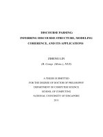
2.2 DHR-PCA (red line) vs. HR-PCA (black line) on the iterative steps
taken by them before convergence with σ = 5 and different dimen-
sionality. The horizontal axis λn is number of corrupted data points
and the vertical axis is the number of steps. Please refer to the color
version. . . . . . . . . . . . . . . . . . . . . . . . . . . . . . . . . . . 34
2.3 DHR-PCA (red line) vs. HR-PCA (black line). m = n = 100, σ =
2. The horizontal axis is the iteration and the vertical axis is the
expressive variance value. Please refer to the color version. . . . . . 35
2.4 DHR-PCA (red line) vs. HR-PCA (black line). m = n = 100, σ =
3. The horizontal axis is the iteration and the vertical axis is the
expressive variance value. Please refer to the color version. . . . . . . 36
2.5 DHR-PCA (red line) vs. HR-PCA (black line). m = n = 100, σ =
10. The horizontal axis is the iteration and the vertical axis is the
expressive variance value. Please refer to the color version. . . . . . . 37
2.6 DHR-PCA (red line) vs. HR-PCA (black line). m = n = 100, σ =
20. The horizontal axis is the iteration and the vertical axis is the
expressive variance value. Please refer to the color version. . . . . . . 38
10
2.7 DHR-PCA (red line) vs. HR-PCA (black line). m = n = 1000, σ =
2. The horizontal axis is the iteration and the vertical axis is the
expressive variance value. Please refer to the color version. . . . . . . 39
2.8 DHR-PCA (red line) vs. HR-PCA (black line). m = n = 1000, σ =
3. The horizontal axis is the iteration and the vertical axis is the
expressive variance value. Please refer to the color version. . . . . . . 40
2.9 DHR-PCA (red line) vs. HR-PCA (black line). m = n = 1000, σ =
10. The horizontal axis is the iteration and the vertical axis is the
expressive variance value. Please refer to the color version. . . . . . . 41

2.10 DHR-PCA (red line) vs. HR-PCA (black line). m = n = 1000, σ =
20. The horizontal axis is the iteration and the vertical axis is the
expressive variance value. Please refer to the color version. . . . . . . 42
2.11 DHR-PCA (red line) vs. HR-PCA (black line). m = n = 10000, σ =
2. The horizontal axis is the iteration and the vertical axis is the
expressive variance value. Please refer to the color version. . . . . . . 43
2.12 DHR-PCA (red line) vs. HR-PCA (black line). m = n = 10000, σ =
3. The horizontal axis is the iteration and the vertical axis is the
expressive variance value. Please refer to the color version. . . . . . . 44
2.13 DHR-PCA (red line) vs. HR-PCA (black line). m = n = 10000, σ =
10. The horizontal axis is the iteration and the vertical axis is the
expressive variance value. Please refer to the color version. . . . . . . 45
2.14 DHR-PCA (red line) vs. HR-PCA (black line). m = n = 10000, σ =
20. The horizontal axis is the iteration and the vertical axis is the
expressive variance value. Please refer to the color version. . . . . . . 46
3.1 Performance comparison of online RPCA (blue line) with online PCA
(red line). Here s = 2, p = 100, T = 10, 000, d = 1. . . . . . . . . . . 64
3.2 Performance of online RPCA. Here s = 3, p = 100, T = 10, 000, d = 1. 64
3.3 Performance of online RPCA. The outliers distribute along 5 different
directions. Here s = 2, p = 100, T = 10, 000, d = 1. . . . . . . . . . . 64
11
4.1 (a) and (b): subspace recovery performance under different corrup-
tion fraction ρ
s
(vertical axis) and rank/n (horizontal axis). Brighter
color means better performance; (c) and (d): the performance com-
parison of the OR-PCA, Grasta, and online PCA methods against
the number of revealed samples under two different corruption levels
ρ
s

with PCP as reference. . . . . . . . . . . . . . . . . . . . . . . . . 105
4.2 The performance comparison of the online RPCA (blue line) on ro-
tating subspaces with the batch RPCA (red lines) method. The un-
derlying subspace is rotated with the parameter δ = 1. . . . . . . . 108
4.3 The performance of the OR-PCA on tracking rotating subspaces un-
der different values of the changing speed parameter δ. . . . . . . . . 109
5.1 Illustration on the importance of the visual word spatial distribution
for image classification purposes. In the top block, the distributions
of a specific visual word in two classes are indicated by circles and
triangles respectively. In the bottom blocks, circles and triangles rep-
resent the pooled statistic values of the two classes. By utilizing the
class-specific local feature spatial distributions, Geometric 
p
-norm
Pooling can generate more separable pooled values, compared with
the average and max pooling. . . . . . . . . . . . . . . . . . . . . . . 112
5.2 Overview of the image classification flowchart. The shown architec-
ture has proven to perform best among the methods based on a single
type of features [85]. Here we replace the original max pooling build-
ing block with our proposed geometric 
p
-norm pooling method, and
shall show the new pipeline is better. . . . . . . . . . . . . . . . . . . 117
12
5.3 Comparison of GLP and average/max pooling over the synthesized
data with distinctive feature distributions for different classes. (a),
(b) and (c), (d) show the exemplar data from two different classes
respectively. (e) displays the optimized geometric coefficients over
the region. Brighter pixels mean that the coefficients are larger at the
corresponding locations. (f) shows the pooling results distribution via

the average, max and GLP poolings. It can be seen that GLP can
separate the data from two classes well while average pooling and
max pooling cannot. . . . . . . . . . . . . . . . . . . . . . . . . . . . 124
5.4 Visualization of the pursued geometric coefficient maps for each spe-
cific visual word over different classes. The left 6 columns show the
exemplar images from 3 classes per dataset and their corresponding
geometric coefficient distribution maps. The coefficients for one spe-
cific class are computed in one-vs-all manner. The right most column
shows the geometric coefficients for one specific visual word, derived
from GLP over all the classes. Each row displays for one dataset. For
better view, please refer to the color version. . . . . . . . . . . . . . 126
6.1 Illustration on the proposed auto-grouped sparse representation method.
The elements of the image-level feature represent different visual pat-
terns. The feature elements are divided into k groups according to
their individual sparse representations. Each group represents one
specific object. Based on the group-wise sparse representations, a
multi-edge graph is constructed to describe the relationship between
the images. . . . . . . . . . . . . . . . . . . . . . . . . . . . . . . . . 131
6.2 Auto-grouped results from ASR on the synthetic datasets for sparse
mixture regression. Top panel shows the 
∞
-distance matrices of
the recovered regression models, where darker color means smaller
distance. And bottom panel shows the convergence curves of the
optimization processes. . . . . . . . . . . . . . . . . . . . . . . . . . . 140
13
6.3 A subgraph of the constructed multi-edge graph. Here 5 types of
features are used. Note that for ease of display, each type of feature
is shown in groups, as indicated by the subscripts in legend. The
groups of these feature elements clusters obtained by ASR are shown

in legend. In the multi-edge graph, the edges’ weights are shown in
a histogram form. . . . . . . . . . . . . . . . . . . . . . . . . . . . . . 143
14
Chapter 1
Introduction
Both research and industry areas (such as engineering, computer science and eco-
nomics) are currently generating terabytes (10
12
bytes) or even petabytes (10
15
bytes) of data in the observations, numerical simulations and experiments. More-
over, the emergence of e-commerce and web search engines has led us to confront the
challenges of even larger scale of data. To be concrete, Google, Microsoft, and other
social media companies (e.g., Facebook, YouTube, Twitter) have data on the order
of exabytes (10
18
bytes) or beyond. Exploring the succinct and relational structure
of the data removes the redundant and noisy information, and thus provides us
with deeper insights into the information contained in the data which benefits our
decision making, users behavior analyzing and prediction.
Actually, analysis of the information contained in these data sets have already
led to major breakthroughs in fields ranging from economics to computer science
and to the development of new information-based industries. However, traditional
methods of analysis have been based largely on the assumption that analysts (e.g.,
the learning and inference algorithms) can work with data within the their limited
computing resources, but the growth of “big data” is imposing great challenges to
them.
More specifically, the challenges raised by “big data” for the machine learning
methods mainly lie on the following two aspects. First, the large scale of the data
causes great storage and computational burdens on the modern sophisticated ma-

15
chine learning, inference and optimization algorithms. Many of existing standard
learning algorithms, though they are statistically performing well, are hindered by
their high computational complexity and do not scale well to the big data. Secondly,
the real data usually contain contamination, which may come from the inherent
noises, corruptions in the measuring or sampling process or even malicious contam-
ination. Such noises and corruptions require the learning methods to possess strong
robustness in order for yielding accurate inference results.
This thesis focuses on the problem of low-dimensional structure learning for big
data analysis. In particular, we investigate and contribute to handling the noise
explosion in the high-dimensional regime and the outliers within the data. Second,
we apply the online learning algorithms to efficiently process the large-scale data
under the limited budget of computational resources. Finally, we demonstrate two
applications of the low-dimensional structure learning methods in object recognition
and image classification.
1.1 Background and Related works
1.1.1 Low-dimensional Structure Learning
Low-dimensional structure represents a more succinct representation of the observed
massive data than their original representation. Finding the low-dimensional struc-
ture of the massive observed data is able to remove the noisy or irrelevant informa-
tion, identify the essential structure of the data and provide us with deeper insight
into the information contained within the data. Moreover, with the help of the
low-dimensional structure mining, we can more conveniently visualize, process and
analyze the data.
Among the traditional low-dimensional structure learning methods, Principal
Component Analysis (PCA) [57] is arguably the most popular one. PCA finds a
low-dimensional subspace which is able to closely fit the observed data, in the sense
of minimizing the square residual error. Following PCA, many other low-dimensional
structure learning methods have been developed based on different criterion in ex-
16

plaining the data. For instance, Locality Preserving Projections (LPP) [122] is pro-
posed to preserve the local relationships among the data after dimension reduction.
Besides linear methods, some non-linear low-dimensional manifold learning meth-
ods are proposed to discover the underlying manifold structure of the data. Typical
examples of those methods include ISOMAP [123], LLE [124], and Laplacian Eigen-
map [125]. Some methods also explore the discriminative low-dimensional structure.
For example, Linear Discriminative Analysis (LDA) [126], or called Fisher Discrimi-
native Analysis (FDA), pursues a linear projection of the data belonging to different
classes in order to maximize the class separability after the linear projection.
Besides pursuing an explicit linear or nonlinear transformation of the data into
low-dimensional structure, some matrix decomposition based method has been pro-
posed to implicitly find the underlying low-dimensional structure. A typical method
is factorizing the data matrix as a low-rank matrix plus a noisy explaining matrix,
where the low-rank factor matrix corresponds to the low-dimensional subspace of
the data [44].
Generally, the methods are batch based and need to load all the data into
memory to perform the inference. This incurs huge storage cost for processing
big data. Moreover, though PCA and other linear methods admit streaming pro-
cessing scheme, it is well known that they are quite fragile to outliers and have weak
robustness.
1.1.2 Robustness in Structure Learning
As discussed above, noises are ubiquitous in realistic data. Traditional low-dimensional
structure learning methods are able to handle the noise with small magnitude in
relatively low-dimensional regime. However, along with the development of mod-
ern data generation and acquisition technologies, the dimensionality of realistic data
keeps increasing. For example, images of much higher resolutions than before can be
acquired rather conveniently. DNA microarray data, financial data, consumer data
also possess quite high dimensionality. In dealing with such high-dimensional data,
the dimensionality explosion is inevitable. However, traditional structure learning
17

methods may fail in this high-dimensional regime [36, 20, 52, 30, 19, 20, 29], due
to their breakdown point being inversely proportional to the dimensionality, or the
unaffordable computational complexity.
Besides the existence of noise in realistic data, some samples or certain dimension
of the data may be corrupted, due to the sensor error or malicious contamination.
The outliers will contaminate the data and manipulate the learning results. In fact,
many of existing low-dimensional structure learning methods, e.g., standard PCA,
are shown to be quite fragile to the outliers. Even one outlier can make the results
arbitrarily bad.
Robustifying the traditional machine learning algorithms becomes a hot and
quite valuable research topic, especially for processing the realistic data with con-
tamination. In particular, many robust learning methods have been proposed for
learning the low-dimensional structure of data [36, 20, 52, 30, 19, 20, 29]. Tradi-
tional machine learning algorithms are generally robustified by employing certain
robust statistics which have high breakdown point. For instance, some of the ex-
isting RPCA methods adopt M-estimator, S-estimator Minimum Covariance Deter-
minant (MCD) estimator to obtain the robust estimation of the sample covariance
matrix. Robust regression based on the robust counterpart of vector inner product
to enhance the robustness, even though there is contamination on the both design
matrix and response variables [127]. Another line of the robust learning is to ex-
plicitly model the added noise on the samples, with certain structural prior, such
as gross though sparse error used in the PCP robust PCA algorithm [44]. In this
thesis, we focus on proposing robust structural learning methods, which can well
handle both the noise in high-dimensional regime and the outliers. In this thesis, we
propose several robust learning methods which are proved to achieve the maximal
robustness.
1.1.3 Online Learning
Online learning is developed for solving the problems where the data are revealed
incrementally over time, and the learner needs to make prediction only based on the
18

data revealed to now, without any knowledge about the coming data in the future.
Online learning originates from game theory, but has been studied in many other
research fields, including information theory and machine learning. Online learning
also becomes of great interest to practitioners due to the recent emergence of large
scale applications such as online advertisement placement and online web ranking.
More formally, online learning is performed in a sequence of consecutive rounds,
where at round t the learner is given a question, x
t
, taken from an instance domain
X, and is required to provide an answer to this question, which we denote by p
t
.
After predicting an answer, the correct answer, y
t
, taken from a target domain Y,
is revealed and the learner suffers a loss, l(p
t
, y
t
), which measures the discrepancy
between its answer and the correct one. The target of the learner is thus to minimize
the cumulative loss

t
l(p
t
, y
t
) or expected loss E
X

l(p
t
, y
t
).
Online learning obviously has the advantages of cheap memory cost in learning
from big data. The online learner only loads one datum or a small batch of the data
into the memory at each time instance, and does not need to re-explore the previous
data in the learning process. In contrast, batch based machine learning algorithms
require to load all the observed data into the memory to perform the parameter
learning and inference. This imposes huge computational burden, especially storage
burden, on the learners and prevents the learners from scaling to big data.
Though they have appealing efficiency advantages, online learning methods often
have quite weak robustness. This is because that the usage of robust statistics for
robustifying the learning methods generally requires statistics over all the data. It
is difficult for the online learning methods which only have a partial observation of
the data to obtain such robust statistics. In this thesis, we investigate and propose
robust online learning algorithms for processing big realistic data.
1.2 Thesis Focus and Main Contributions
In this thesis, we focus on robust and efficient low-dimensional structure learning
for big data analysis. The main motivations are as follows:
19
1. For more efficient batch high-dimensional RPCA algorithm. Big data often
have high dimensionality. In the high-dimensional regime, noise explosion will
destroy the signal and fail many existing low-dimensional subspace learning
method. A strategy to handle the noise and outliers is to introduce randomness
on the sample selection. However, such method is quite inefficient as only at
most one sample is removed in each optimization iteration. A deterministic
method is desired for providing high efficiency.
2. With limited budget of memory, how to handle the large-scale dataset. For

common users, the computational budget is usually limited. However, tra-
ditional machine learning methods are generally batch based, which require
to load all the data into memory. This is the bottleneck for processing big
data. Therefore, an online learning algorithm which processes the data in a
streaming manner and meanwhile preserves the desired property of the batch
methods is required.
3. We are also interested in the application of the low-dimensional structure
learning method in real applications. In particular, we focus on solving the
problem of object recognition in computer vision research field. The discovered
low-dimensional structure is able to convey more essential and discriminative
information for classification. Thus, based on such structure, more discrim-
inative image representations can be obtained which are more beneficial for
image classification and/or object recognition.
In this thesis, the robust low-dimensional structure learning method, especially
for the low-dimensional subspace learning, is proposed. Furthermore, we successfully
scale the method to big data regime via proposing the online learning method. We
also apply the low-dimensional learning method on computer vision applications.
More specifically, we conduct research on the following aspects:
1. Deterministic high-dimensional robust PCA method. We first develop a deter-
ministic robust PCA method for recovering low-dimensional subspace of high-
20
dimensional data, where the dimensionality of each datum is comparable or
even larger than the number of data. The DHRPCA method is tractable, pos-
sesses maximal robustness, and asymptotic consistent in the high-dimensional
space. More importantly, by smartly suppressing the affect of outliers in a
batch manner, the method exhibits significantly high efficiency for handling
large-scale data.
2. Online robust PCA methods.
Second, we propose two online learning methods, OR-PCA and online RPCA,
to further enhance the scalability for robustly learning the low-dimensional

structure of big data, under limited memory and computational cost bud-
get. These two methods handle two different types of contaminations within
the data: (1) OR-PCA is for the data with sparse corruption and (2) online
RPCA is for the case where a few of the data are completely corrupted. In
particular, OR-PCA introduces a matrix factorization reformulation of nuclear
norm which enables alternative stochastic optimization to be applicable and
converge to the global optimum. Online RPCA devises a randomized sample
selection mechanism which possesses provable recovering performance and ro-
bustness guarantee under mild condition. Both of these two methods process
the data in a streaming manner and thus are memory and computationally
efficient for analyzing big data.
3. The applications in computer vision tasks. Furthermore, we devise two low-
dimensional learning algorithms for visual data and solve several important
problems in computer vision: (1) geometric pooling which generates discrim-
inative image representation based on the low-dimensional structure of the
object class space, and (2) auto-grouped sparse representation for discover-
ing low-dimensional sub-group structure within visual features to generate
better feature representations. These two methods achieve state-of-the-art
performance on several benchmark datasets for the image classification, image
annotation and motion segmentation tasks.
21
1.3 Structure of The Thesis
In Chapter 2, we propose a deterministic robust PCA method for learning the low-
dimensional structure of data in high-dimensional regime. Then in Chapter 3 and
Chapter 4, we propose two different online robust PCA methods to handle data
with different corruption models. Finally, we demonstrate two applications of the
low-dimensional structure learning in object recognition and image annotation tasks
in Chapter 5 and Chapter 6.
22
Chapter 2

Robust PCA in High-dimension:
A Deterministic Approach
In this chapter, we propose our robust PCA method for handing the data with
quite high dimensionality and meanwhile a subset of the data is corrupted to be
outliers. We propose a deterministic algorithm which is much more efficient than
its randomized counterpart yet possesses the maximal robustness.
2.1 Introduction
This chapter is about robust principal component analysis (PCA) for high-dimensional
data, a topic that has drawn surging attention in recent years. PCA is one of the
most widely used data analysis methods [57]. It constructs a low-dimensional sub-
space based on a set of principal components (PCs) to approximate the observations
in the least-square sense. Standard PCA computes PCs as eigenvectors of the sam-
ple covariance matrix. Due to the quadratic error criterion, PCA is notoriously
sensitive and fragile, and the quality of its output can suffer severely in the face of
even few corrupted samples. Therefore, it is not surprising that many works have
been dedicated to robustifying PCA [52, 20, 44].
Analyzing high dimensional data – data sets where the dimensionality of each
observation is comparable to or even larger than the number of observations – has
23
become a critical task in modern statistics and machine learning [6]. Practical high
dimensional data, such as DNA microarray data, financial data, consumer data, and
climate data, easily have dimensionality ranging from thousand to billions. Partly
due to the fact that extending traditional statistical tools (designed for the low
dimensional case) into this high-dimensional regime are often unsuccessful, tremen-
dous research efforts have been made to design fresh statistical tools to cope with
such “dimensionality explosion”.
The work in [61] is among the first to analyze robust PCA algorithms in the high-
dimensional setup. They identified three pitfalls, namely diminishing breakdown
point, noise explosion and algorithmic intractability, where previous robust PCA
algorithms stumble. They then proposed the high-dimensional robust PCA (HR-

PCA) algorithm that can effectively overcome these problems, and showed that
HR-PCA is tractable, provably robust and easily kernelizable. In particular, in
contrast to standard PCA and existing robust PCA algorithms, HR-PCA is able
to robustly estimate the PCs in the high-dimensional regime even in the face of
a constant fraction of outliers and extremely low Signal Noise Ratio (SNR) – the
breakdown point of HR-PCA is 50%,
1
which is the highest breakdown point can ever
be achieved, whereas other existing methods all have breakdown points diminishing
to zero. Indeed, to the best of our knowledge, HR-PCA appears to be the only
algorithm having these properties in the high-dimensional regime.
Briefly speaking, HR-PCA is an iterative method which in each iteration per-
forms standard PCA, and then randomly remove one point in a way that outliers
are more likely to be removed, so that the algorithm converges to a good output.
Because in each iteration, only one point is removed, the number of iterations re-
quired to find a good solution is at least as much as the number of outliers. This,
combined with the fact that PCA is computationally expensive itself, prevents HR-
PCA from effectively handling large-scale data-sets with many outliers. In addition,
the performance of HR-PCA depends on the ability of the built-in random removal
1
Breakdown point is a robustness measure defined as the percentage of corrupted points that
can make the output of the algorithm arbitrarily bad.
24