Advanced measurement techniques in optical fiber sensor and communication systems
Bạn đang xem bản rút gọn của tài liệu. Xem và tải ngay bản đầy đủ của tài liệu tại đây (3.09 MB, 153 trang )
ADVANCED MEASUREMENT TECHNIQUES IN OPTICAL
FIBER SENSOR AND COMMUNICATION SYSTEMS
HU JUNHAO
NATIONAL UNIVERSITY OF SINGAPORE
2011
ADVANCED MEASUREMENT TECHNIQUES IN OPTICAL
FIBER SENSOR AND COMMUNICATION SYSTEMS
HU JUNHAO
(B. Eng., Huazhong University of Science and Technology, China)
A THESIS SUBMITTED
FOR THE DEGREE OF DOCTOR OF PHILOSOPHY
DEPARTMENT OF ELECTRICAL AND COMUPTER
ENGINEERING
NATIONAL UNIVERSITY OF SINGAPORE
2011
Acknowledgement
Many people have inspired, guided and helped me during my four years PhD study in
National University of Singapore. I would like to thank them all.
Firstly, I would like to give my special thanks to my supervisor, Dr. Changyuan Yu, for
his professional guidance and enthusiastic support during my PhD study. It is him who
has opened the door of research and illuminates my future. In the last four years,
sometimes, I might feel depressed and lose the confidence to continue my PhD study; it is
him who encouraged me and gave me the confidence to continue.
And I also want to thank Dr. Chen Zhihao for his help on my research in optical fiber
sensor systems. He gave me a lot of guidance and help on the experiment of long distance
FBG sensor system. He gave me the direction of research on how to improve the
performance of experiment. Without his help, I cannot finish this project.
I am also fortunate enough to work with many outstanding students and research staffs in
our group. I take this opportunity to thank Dr. Yang Jing for her beneficial suggestions
and encouragement in my study and life.
Finally, my deepest gratitude goes to my parents. Their support and encouragement are
always here whenever I encounter any difficulties. And I also want to thank my girlfriend
for her support.
With their help, my PhD experience has been the most rewarding and pleasant.
i
Table of Content
Acknowledgement .............................................................................................................. i
Table of Content ................................................................................................................ ii
Summary ........................................................................................................................... vi
List of Figures .................................................................................................................... x
List of Tables ................................................................................................................... xvi
List of Abbreviations ..................................................................................................... xvii
1 Introduction .................................................................................................................... 1
1.1 Pulse generation and measurement techniques ................................................................. 3
1.1.1 Pulse train generation using SWNTs as saturable absorber............................................. 4
1.1.2 Pulse measurement techniques ........................................................................................ 4
1.1.3 Limitation of conventional second-harmonic generation autocorrelator......................... 7
1.2 Review of optical fiber sensors ............................................................................................ 8
1.2.1 Fiber Bragg grating sensor system ................................................................................ 11
1.2.2 Long distance FBG sensor system ................................................................................ 14
1.3 Performance monitoring in optical communication system ........................................... 15
1.4 Focus and structure of the thesis....................................................................................... 18
2 Pulse Generation based on Carbon Nano-tube fiber laser ....................................... 20
2.1 Background and methods .................................................................................................. 21
2.1.1 Working principle of Q-switched laser system ............................................................. 21
ii
2.1.2 Fabricating single-wall nanotube saturable absorber with low insertion loss ........... 24
2.2 Tunable wavelength CNT-SAs Q-switched fiber ring laser ............................................ 26
2.3 Tunable wavelength, tunable repetition rate linear cavity CNT-SAs Q-switched fiber
laser ........................................................................................................................................... 31
2.3.1 Experimental setup of the linear cavity fiber laser ........................................................ 32
2.3.2 Experimental results and discussions ............................................................................ 33
2.4 Tunable repetition-rate FBG linear cavity CNT-SAs Q-switched fiber laser ............... 36
2.4.1 110-cm length FBG linear cavity fiber laser setup ........................................................ 37
2.4.2 Experimental results and discussions ............................................................................ 38
2.5 Comparison ......................................................................................................................... 41
3 Pulse measurement based on degree of polarization (DOP) autocorrelation method
........................................................................................................................................... 44
3.1 Experiment setup and operation principle ...................................................................... 46
3.2 Simulation results ............................................................................................................... 48
3.2.1 Chirp effect to the pulse width measurement ................................................................ 48
3.2.2 Misalignment effect to the pulse width measurement ................................................... 53
3.3 Experimental results .......................................................................................................... 55
3.4 Comparison and conclusions ............................................................................................. 57
4 Long distance fiber Bragg grating sensor system based on Raman amplification 60
4.1 Background and operation principle ................................................................................ 62
4.1.1 Spontaneous vs. stimulated Raman scattering ............................................................... 62
4.1.2 Operation principle of 100-km long distance fiber Bragg grating sensor ..................... 66
4.1.3 Operation principle of 150-km long distance fiber Bragg grating sensor ..................... 68
iii
4.2 150-km multi-point temperature and vibration sensor system ...................................... 70
4.2.1 Multi-point long distance FBG sensor system .............................................................. 70
4.2.2 Long distance temperature sensor system ..................................................................... 73
4.2.3 Long distance vibration sensor system .......................................................................... 75
4.2.3.1 Vibration sensor based on tunable filter ................................................................................75
4.2.3.2 Vibration sensor system based on matching filter demodulation ..........................................76
4.2.3.3 Experiment results of vibration sensor system ......................................................................79
4.3 Conclusions ......................................................................................................................... 80
5 CD monitoring based on delay tap sampling with low bandwidth receiver ........... 81
5.1 Principle of Delay-tap Sampling Plot ............................................................................... 83
5.2 Delay tap sampling methods based on low bandwidth balanced receiver of 50-Gbit/s
RZ-QPSK signal ....................................................................................................................... 86
5.2.1 Simulation results .......................................................................................................... 86
5.2.2Experiment results of using low bandwidth balanced receiver ...................................... 89
5.2.3 Comparison between the results of high bandwidth balanced receiver and our method
................................................................................................................................................ 92
5.3 Delay tap sampling method based on single low bandwidth receiver ........................... 95
5.3.1 Simulation results based on one low bandwidth receiver.............................................. 96
5.3.2 Experiment results of using a single low bandwidth receiver ....................................... 98
5.3.3 Comparison between high bandwidth receiver and our method ................................. 100
5.3.3.1 Simulation results of CD monitoring scheme using one 40-GHz bandwidth receiver ........ 101
5.3.3.2 Experiment results of CD monitoring scheme using one 40-GHz bandwidth receiver....... 101
5.4 Conclusions ....................................................................................................................... 103
6 Conclusions and Future Works ................................................................................ 104
iv
6.1 Conclusions ....................................................................................................................... 104
6.2 Future Works .................................................................................................................... 106
6.2.1 Improvement on autocorrelator based on DOP measurement ..................................... 106
6.2.2 Improvement on the long distance FBG sensor system. ............................................. 107
6.2.3 Improvement on CD monitoring system based on low bandwidth delay tap sampling
method. ................................................................................................................................. 107
Bibliography .................................................................................................................. 109
Publication list ............................................................................................................... 130
v
Summary
In 1870, John Tyndall demonstrated that light can follow a specific path by using internal
reflection. This is the first concept that fiber can be used to guide the light. As the
development of fiber, glass fiber is proposed. However, the losses of these fibers are too
large to transmit signals over long distance fibers. Later, in 1960s, Charles Kao and his
co-workers demonstrated that the high-loss of fiber comes from impurities in the glass,
not the glass itself. From this concept, using fiber as a telecommunication medium has
been realized. Optical fiber has a lot of applications; and the two main applications are
optical fiber communication and fiber optic sensors.
However, there are still many problems to be solved in these two main
applications. For optical fiber communication system, there are a lot of effects that can
affect the system performance, such as the chromatic dispersion (CD), polarization mode
dispersion (PMD), optical signal noise ratio (OSNR) and other nonlinear effects. In order
to improve the performance, many techniques are proposed to monitor and measure these
effects. Taking CD monitoring as an example, there are radio frequency power fading
method, additional pilot tone method, delay-tap sampling plots method and others. For
the fiber optic sensor system, there are also a lot of problems to be solved. Take the gas
and oil pipeline leakage monitoring sensor as an example; it should be long distance, high
vi
robustness and low cost. In this thesis, several advanced measurement techniques in
optical fiber communication and fiber optic sensor systems are introduced.
Firstly, pulse train generation and measurement techniques are introduced. Qswitched single wall nanotubes (SWNTs) fiber laser with low insertion loss is firstly
demonstrated in this thesis. As we know, a saturable absorber is the key component of
passive Q-switched laser to generate the pulse trains. These saturable absorbers are
normally semiconductor saturable absorber and crystal saturable absorber, which is not
friendly using to fabricate all-fiber lasers. Later, in 2008, SWNTs is firstly used to
generate a tunable wavelength mode-locked fiber laser; and it is published on Nature
Nanotechnology. Nowadays, SWNTs are widely used to generate ultra-short pulse width
mode-locked lasers. But Q-switched SWNTs all-fiber lasers have never been
demonstrated before. In this thesis, we firstly reduce the SWNTs insertion loss from 3 dB
to 0.7 dB. Then we introduce three different SWNTs based Q-switched fiber lasers. They
are C+L band tunable wavelength SWNTs all-fiber ring laser, tunable wavelength tunable
repetition rate linear cavity SWNTs fiber laser and tunable repetition rate FBG linear
cavity SWNTs fiber laser.
After introducing the pulse generation based on SWNTs, a low power
autocorrelator is proposed based on degree of polarization (DOP) measurement. Firstly,
the chirp factor and mismatching angle is studied in simulation. It is found that the pulse
widths almost have the linear relationship with the chirp factors, which means our
method can be used to measure the chirp factor if the original pulse width is known. And
vii
the small effects of mismatching angle on pulse width measurements prove the high
misalignment tolerance of the system. Compared with the traditional second harmonic
generation (SHG) autocorrelator, which requires very rigid alignment and high laser
power, this method can measure -60 dBm power pulse train with shorter time. The
sensitivity of our method has been increased to 10-20 W2, compared with the SHG
autocorrelator 10-7 W2.
After introducing the pulse width measurement, the measurement techniques in
fiber optic sensor system are introduced. As we know, there are many problems in the
fiber optic sensor system, such as the measurement length, cost and robustness. In this
thesis, a simple and cost effective method is proposed to solve the measurement length
issue of the FBG sensor systems. A novel 150-km multi-point long distance FBG
temperature and vibration fiber sensing system is demonstrated based on Raman
amplification. In addition to a Raman laser at 1395 nm and a laser at 1480 nm, the 150km long distance system is constructed only by passive optical components, such as the
coupler, SMF and EDF. It is an all fiber long distance temperature and vibration sensor
system without any electrical components along the 150-km fiber. The accuracy of this
temperature sensor is about 1 oC; and the vibration measurement range is from 1 Hz to
1000 Hz.
After introducing the measurement techniques in fiber optic sensor systems,
measurement techniques in optical communication system is also introduced, especially
in chromatic dispersion (CD) monitoring. There are many CD monitoring techniques,
viii
such as the radio frequency power fading method, additional pilot tone method and delaytap sampling plots method. In this thesis, in the specific techniques of CD monitoring, a
low bandwidth receiver delay-tap sampling method is demonstrated and proved to have
better performance than the high cost high bandwidth receiver delay-tap sampling method.
Firstly, both the low bandwidth and high bandwidth balanced receiver are compared to
demodulate the 50-Gbit/s RZ-QPSK signals and generate delay-tap sampling plots. It is
proved that the low cost low bandwidth balanced receiver has increased the CD
measurement range and the sensitivity in small CD range. Then we also find that one
single low bandwidth photo-detector can achieve the same performance as balanced
receiver. It is obvious that a single low bandwidth photo-detector is more welcomed for
its low cost and simplicity. After comparing the simulation and experiment results, the
consistent between them proves that our proposed low bandwidth receiver method has
not only provided larger measurement range and sensitivity, but also reduced the cost of
the system.
ix
List of Figures
Fig. 1.1 The setup of intensity autocorrelator. .................................................................... 7
Fig. 1.2 Distribution of OFS-15 papers according to measurands [13]. ........................... 10
Fig. 1.3 Distribution of fiber optics sensors according to technologies [13]. ................... 10
Fig. 1.4 Types of fiber gratings: (a) fiber Bragg grating, (b) long-period fiber grating, (c)
chirped fiber grating, (d) tilted fiber grating. .................................................................... 12
Fig. 2.1 (a) Q-switching operation principle, (b) Actively Q-switched setup, (c) Passively
Q-switched setup. .............................................................................................................. 23
Fig. 2.2 Setup for depositing carbon nanotubes on the ends of cleaved optical fibers using
optical radiation [75]. Forces due to optical radiation are also shown. ............................ 25
Fig. 2.3 Using mechanical connector to fabricate low insertion loss SWNTs in the system.
........................................................................................................................................... 25
Fig. 2.4 Experiment setup of the wideband-tunable fiber laser. ....................................... 26
Fig. 2.5 Generated pulse train by using (a) 0.5 nm bandwidth filter (b) 2 nm bandwidth
filter ................................................................................................................................... 27
Fig. 2.6 Spectra output at 1570 nm under different pump powers with (a) 0.5-nm
bandwidth filter (b) 2-nm bandwidth filter ....................................................................... 29
Fig. 2.7 Output power and pulse repetition rate as a function of pump power at 1570 nm
with (a) 0.5-nm bandwidth filter (b) 2-nm bandwidth filter ............................................. 29
Fig. 2.8 Laser output spectra at different wavelengths under pump power of 35.94 mW. 30
Fig. 2.9 Pulse output power and repetition rate under different wavelengths .................. 31
x
Fig. 2.10 Experiment setup of low-threshold linear cavity tunable erbium-doped fiber
laser. .................................................................................................................................. 32
Fig. 2.11 Output spectra of the fiber laser at different pump powers. .............................. 33
Fig. 2.12 Pulse trains in time domain under the pump powers of (a) 18.57 mW and (b)
118.8 mW. ......................................................................................................................... 33
Fig. 2.13 Pulse repetition rate and average output power as functions of the pump power.
........................................................................................................................................... 35
Fig. 2.14 Laser output spectra at different wavelengths under a pump power of 45.01 mW.
........................................................................................................................................... 35
Fig. 2.15 Laser output power and pulse-repetition-rate under different wavelengths. ..... 36
Fig. 2.16 110-cm length FBG linear cavity fiber laser setup. ........................................... 37
Fig. 2.17 Output spectrum under difference pump powers............................................... 38
Fig. 2.18 Pulse train under pump powers (a) 29.85 mW and (b) 76.82 mW. ................... 38
Fig. 2.19 Pulse train under pump powers (a) 120.7 mW and (b) 152.3 mW .................... 39
Fig. 2.20 Measured pulse width under pump powers of 152.3 mW ................................. 40
Fig. 2.21 Measured pulse duration under different pump powers .................................... 40
Fig. 2.22 Pulse repetition rate and average output power as functions of pump power. .. 41
Fig. 3.1 (a) Experimental setup, (b) The illustration of pulse property at different
locations of the component corresponding to the experimental setup. ............................. 47
Fig. 3.2 Simulation results of the autocorrelation function with the chirp factor α from 0
to 1 for (a) 5-ps Gaussian pulse train and (b) 15-ps Gaussian pulse train. ....................... 49
Fig. 3.3 Simulation results of the autocorrelation trace with the chirp factor α from 0 to 5
xi
for 5-ps Gaussian pulse (b) 15-ps Gaussian pulse. ........................................................... 51
Fig. 3.4 Chirp effect on pulse width measurement for 2-ps, 5-ps, 10-ps, and 15-ps
Gaussian pulse trains......................................................................................................... 52
Fig. 3.5 Simulation results of the alignment angle to the tunable DGD component from
45o to 50o (a) for 5-ps Gaussian pulse train and (b) for 15-ps Gaussian pulse train. ........ 54
Fig. 3.6 The misalignment effect on pulse width measurement for 2-ps, 5-ps, 10-ps and
15-ps pulse width Gaussian pulse trains. .......................................................................... 55
Fig. 3.7 Experimental measured pulse widths of 10-GHz pulse train: (a) 5.11 ps pulse
width by using our method; and (b) 5.06 ps by using SHG autocorrelation. ................... 56
Fig. 3.8 Comparison between pulse-width from conventional SHG autocorrelator and
pulse-width measured by our method. .............................................................................. 58
Fig. 4.1 Experiment setup to illustrate spontaneous Raman scattering in long distance
sensor system. ................................................................................................................... 64
Fig. 4.2 Transmitted spectrum of experiment setup in Fig. 4.1. The power of 1395-nm
laser is 27 dBm.................................................................................................................. 64
Fig. 4.3 Experiment setup to illustrate stimulated Raman scattering in our new proposed
long distance sensor system. ............................................................................................. 65
Fig. 4.4 Transmitted spectrum of experiment setup in Fig. 4.3. The power of 1395-nm
laser and 1480-nm laser is 27 dBm and 3.3 mW............................................................... 66
Fig. 4.5 Experiment setup to illustrate the working principle of the 100-km long distance
FBG sensor system. .......................................................................................................... 67
Fig. 4.6 Transmitted spectrum of the setup in Fig. 4.5. .................................................... 68
xii
Fig. 4.7 Experimental setup for illustrating the working principle of 150-km FBG sensor
system. .............................................................................................................................. 69
Fig. 4.8 Transmitted spectrum of the setup in Fig. 4.7. .................................................... 69
Fig. 4.9 150-km multi-point FBG temperature and vibration sensor system. .................. 70
Fig. 4.10 Reflected spectrum of the system at the range from 1551 nm to 1562 nm. ...... 72
Fig. 4.11 Reflected spectra of FBG Bragg wavelengths at four different temperatures. .. 73
Fig. 4.12 FBG Bragg wavelengths as a function of the applied temperatures .................. 74
Fig. 4.13 The spectrum after the tunable filter, (a) with no strain on the FBG (Dashed
line); (b) with the maximum strain on the FBG (Solid line)............................................. 76
Fig. 4.14 Experiment setup of using matching filter demodulation. ................................ 77
Fig. 4.15 Matching FBG pair demodulation. .................................................................... 78
Fig. 4.16 Recorded waveform on the oscilloscope when vibration frequency is 13 Hz... 79
Fig. 4.17 Detected frequency displayed on computer after FFT when vibration frequency
is set on (a) 1.5 Hz, (b) 100 Hz, (c) 500.5 Hz, (d) 1000 Hz.............................................. 80
Fig. 5.1 Principle of delay-tap asynchronous sampling for RZ-QPSK signal. (a) schematic
graph of delay sampling (b) waveforms in the time domain; (c) eye diagram; (d) delaytap plot using low bandwidth receiver. (∆t=symbol period/2). Ts: sampling period; ∆t:
time offset. ........................................................................................................................ 85
Fig. 5.2 System setup of CD monitoring scheme of 50-Gbit/s RZ-QPSK signal. ............ 86
Fig. 5.3 Delay-tap sampling plots with different residual CD when using a 12-GHz
balanced receiver. .............................................................................................................. 87
Fig. 5.4 Simulation Result of amplitude ratio as a function of residual CD when a 12-
xiii
GHz bandwidth balanced receiver is used. ....................................................................... 88
Fig. 5.5 Experiment setup of CD monitoring method in 50-Gbit/s RZ-QPSK systems. .. 89
Fig. 5.6 (a) Balanced receiver eye diagram without filter when CD=0 ps/nm(b) Balanced
receiver eye diagram with filter when CD=0 ps/nm. ........................................................ 89
Fig. 5.7 Delay tap sampling plot of different residual CD. ............................................... 90
Fig. 5.8 Comparison between the experiment and simulation results. ............................. 91
Fig. 5.9 Experiment setup of CD monitoring method in [147] using normal bandwidth
balanced receiver. .............................................................................................................. 92
Fig. 5.10 Delay tap sampling plots with different CDs when using the 40-GHz receiver.93
Fig. 5.11 Experiment results of traditional method that use normal bandwidth balanced
receiver. ............................................................................................................................. 95
Fig. 5.12 Delay taped sampling system setup for CD monitoring based on single low
bandwidth receiver. SMF: single mode fiber; MZI: Mach–Zehnder interferometer; PD:
photo-detector; GND: ground. .......................................................................................... 96
Fig. 5.13 Delay-tap sampling plots with different values of CD when using one low
bandwidth single detector. ................................................................................................ 97
Fig. 5.14 Relationship between CD and amplitude ratio. ................................................. 98
Fig. 5.15 Delay-tap sampling plots of experiment results. ............................................... 99
Fig. 5.16 Relationship between chromatic dispersion and amplitude ratio of experiment
and simulation results. .................................................................................................... 100
Fig. 5.17 Delay taped sampling system setup based on single high bandwidth photodetector. ........................................................................................................................... 100
xiv
Fig. 5.18 Delay tap sampling plots of 40-GHz receiver. ................................................ 101
Fig. 5.19 Delay-tap sampling plots by using one normal bandwidth receiver. ............... 102
Fig. 6.1 Delay tap sampling plots when using the 3-order Bessel low band pass filter, (a)
when CD is 120 ps/nm and (b) when CD is -120 ps/nm. ............................................... 108
xv
List of Tables
Table 1. Comparison between three different setups. ....................................................... 43
Table 2. Power measurement in different pulse widths .................................................... 59
xvi
List of Abbreviations
ASE
Amplified Stimulated Emission
BER
Bit Error Rate
CD
Chromatic Dispersion
CDMA
Code Division Multiple Access
CNT-SAs
Carbon Nanotube Saturable Absorbers
CSRZ
Carrier Suppressed Return-to-Zero
CW
Continuous Wave
DAQ
Data Acquisition
DFB
Distributed Feedback
DGD
Differential Group Delay
DOP
Degree-of-Polarization
DQPSK
Differential Quadrature Phase-Shift Keying
DWDM
Dense Wavelength-Division-Multiplexing
EDF
Erbium Doped Fiber
EDFL
Erbium Doped Fiber Laser
EMI
Electromagnetic Interference
FBG
Fiber Bragg Grating
FFT
Fast Fourier Transform
xvii
FM
Frequency Modulated
FROG
Frequency-Resolved Optical Gating
FWHM
Full-Width at Half-Maximum
GND
Ground
ISO1
Isolators
LPG
Long-Period Grating
MZI
Mach-Zehnder Interferometer
NI
National Instrument
OC
Optical Circulators
OFS
Optical Fiber Sensors
OSA
Optical Spectrum Analyzer
OSNR
Optical Signal-to-Noise Ratio
OTDRs
Optical Time-Domain Reflectometers
PBC
Polarization Beam Combiner
PC
Polarization Controller
PD
Phtotodector
PMD
Polarization Mode Dispersion
PSP
Principal-States-of-Polarization
PBS
Polarization Beam Splitters
QPSK
Quadrature Phase-Shift Keying
RF
Radio-Frequency
RZ
Return-to-Zero
xviii
SAs
Saturable Absorbers
SDM
Spatial Division Multiplexing
SESAMs
Semiconductor Saturable Absorber Mirrors
SHB
Spatial Hole Burning
SHG
Second-Harmonic Generation
SI
Spectral Interferometry
SMF
Single Mode Fiber
SNR
Signal-to-Noise Ratio
SOP
State-of-Polarization
SPIDER
Spectral Phase Interferometry for Direct Electric-field
Reconstruction
SRS
Stimulated Raman Scattering
SWNTs
Single Walled Nanotubes
TDM
Time Division Multiplexing
VOA
Variable Optical Attenuator
WDM
Wavelength Division Multiplexing
xix
Chapter 1
Introduction
As we know, Daniel Colladon and Jacques Babinet firstly demonstrated the concept of
fiber in 1840s. 12 years later, John Tyndall demonstrated it in his public lectures in
London. In 1960s, Charles Kuen Kao (The 2009 Nobel Prize winner in Physics)
published that the high loss of existing fiber arose from the impurities in the glass, rather
than from the technology itself. Charles Kuen Kao and his coworkers did their pioneering
work to make the realization of using fiber as a telecommunications medium. Due to the
evolution of fiber fabrication, the loss of fiber has been reduced to 0.2 dB/km. This big
improvement changes our world greatly in last 30 years. Because of this invention, our
world is becoming a truly global village after implementing optic fiber in optical
communication systems. These telecommunication links between the countries provide
us low price, high speed and high bandwidth Internet. It supports all the global business,
1
finance, market, and communication.
In parallel with the application of optical fiber communication, optical fiber has
another main application, fiber optic sensors. They cover a lot of sensor areas, such as
the rotation, acceleration, electric and magnetic field measurement, temperature, pressure,
acoustics, vibration, linear and angular position, strain, humidity, viscosity, chemical
measurements and so on. They can replace many traditional sensors and provides better
quality and performance at the same time. All these good performances come from the
inherent advantages of the optical fiber, which includes (1) lightweight and small size, (2)
passive, (3) low power, (4) resistant ability to electromagnetic interference, (5) high
sensitivity, (6) large bandwidth and (7) environmental ruggedness.
Moreover, a lot of useful components associated with optical fiber communication
are demonstrated for fiber optic sensor applications. Fiber optic sensor technologies, in
turn, are driven by the development and subsequent mass production of components to
support optical communication. In the specific area of measurement technology of optical
fiber sensor and communication systems, great demands are needed in the market. For
example, in optical communication systems, a lot of parameters should be measured and
monitored, such as power, loss, dispersion, bit-error rate (BER), signal-noise-ratio (SNR)
and so on. Measurement of these parameters is required to provide feedback to the system
and sustain a stable and high quality performance. In addition, in the optical sensor
system, lots of parameters are also needed to be measured in the application areas, such
as temperature, strain, rotation, humidity, vibration and so on.
In this chapter, backgrounds of these advanced measurement techniques are
introduced. Firstly, pulsed laser techniques and pulse measurement techniques are
2
discussed in section 1.1. The optical fiber sensor techniques, especially the fiber Bragg
grating sensors, are reviewed in section 1.2. The performance monitoring techniques in
optical communication system, especially the chromatic dispersion is introduced in
section 1.3. The outline and objective of this thesis are presented in section 1.4.
1.1 Pulse generation and measurement techniques
As we know, laser can be generated if three conditions are satisfied: gain medium, cavity
and population conversion. If pulsed laser is given, two parameters are commonly used to
characterize them. The first one is the average output power:
Pave =Epulse*Rrepetition
(1.1)
The second one is the peak power, which may be approximated as follows:
Ppeak
E pulse
t
(1.2)
where Epulse is the energy per pulse, t is the FWHM of the pulse.
As we know, there are several approaches to pulsing lasers [1]:
1. Pulse the excitation itself, such as using modulators.
2. Mode locking.
3. Q-switching.
Compared to the mode-locking methods of generating pulsed laser, Q-switched
method is relatively simple. The pulse generated Q-switched method typically has larger
than 1 ns pulse width. However, it has several advantages:
a. Cost effective
b. Easy to implement
3
c. Efficient in extracting energy stored in upper laser level.
In this thesis, several Q-switched fiber laser systems are proposed by using SWNTs,
which will be illustrated in chapter 2.
1.1.1 Pulse train generation using SWNTs as saturable absorber
Saturable absorber is an optical component, whose loss can decrease at high optical
intensities. For example, in a medium with absorbing dopants ions, this situation occurs
when a strong optical intensity leads to depletion of the ground state of these ions. In
semiconductor, the excitation of electrons from the valence band into the conduction
band reduces the absorption for photon energies just above the band gap energy. These
saturable absorbers are the key component to generate mode-locked and Q-switched
lasers. Because of the simplicity and cost efficiencies of all-fiber lasers, simple and low
cost saturable absorbers attract significant attentions. Before the introduction of single
walled Nanotubes (SWNTs), semiconductor saturable absorber mirrors (SESAMs) are
widely used [2, 3]. But they are expensive and complex to construct in the laser setup.
After the introduction of SWNTs, they are often used in the system to achieve ultra-short
pulsed lasers, such as the first tunable wavelength SWNTs mode-locking fiber lasers [4].
However, SWNTs have rarely been used to generate Q-switched pulse trains. Recently, a
simple Q-switched fiber laser with SWNTs is demonstrated [5].
1.1.2 Pulse measurement techniques
As we know, the short pulse width measurement is a big issue. For the Q-switched pulse
trains that normally have larger than 1 ns pulse width, the photodiodes and oscilloscopes
can measure the pulse width of these pulse trains. How can we measure the pulse trains
4