Bioanalytical strategies for the quantification of xenobiotics in biological fluids and tissues 3
Bạn đang xem bản rút gọn của tài liệu. Xem và tải ngay bản đầy đủ của tài liệu tại đây (947.34 KB, 32 trang )
Chapter 3
Chapter 3 Biomonitoring of environmental organic
pollutants in human ovarian tumor cyst fluids samples using
µ-SPE-GC-MS and HPLC-florescence detection and
principal component analysis
Chapter 3
44
3.1 Preface to Chapter 3
To assess a possible etiological role of environmental organic pollutants in
ovarian cancer development on ovarian cancer patients, concentrations of different
groups of organic pollutants were measured in 20 malignant and benign ovarian cyst
fluid samples of women with ovarian cancer. A total of 60 chemicals of six groups
including heterocyclic aromatic amines, Low molecular weight organic acids,
aromatic amines, N-nitrosamines, Polybrominated diphenyl ethers and halogenated
flame retardants and organochlorine pesticides were assayed via porous membrane
protected micro-solid-phase extraction followed by GC-MS detection and HPLC-
fluorescence detection. High performance liquid chromatography coupled with
fluorescence detection was used to quantify heterocyclic aromatic amines and
aromatic amines. Gas chromatography-mass spectrometry was used to quantify
PBDEs and halogenated flame retardants, and LMW organic acids. Trace amounts of
most of the chemicals were found both in benign and malignant cyst fluid samples.
The trend in their concentration in benign and malignant samples was projected by
principal component analysis using R program. The results reveal that the possible
correlations in the concentration of chemicals with the malignancy of the ovarian
tumour.
Chapter 3
45
3.2 Introduction
Ovarian cancer is the fifth most common cancer among women worldwide and
is the fourth most common cancer in Singapore [1]. It causes more deaths than any
other type of female reproductive cancer. The risk for developing ovarian cancer
appears to be affected by several factors. Exposure to endocrine disruptive
xenobiotics is recognized as an important environmental risk factor associated with
development of cancer.
Global epidemiologic studies have indentified environmental and occupational
chemicals as potential carcinogens. Many studies provide the direct association
between these chemicals, especially EDCs with the development of different types of
gynaecological cancer [2]. Many environmental chemical contaminants, which may
also be the metabolic intermediates, particularly those that are lipophilic and of
relatively low molecular weight, can accumulate in tissue and body fluids. The
potential health effects of these contaminants on human are of great concern, making
it important to carefully monitor their levels and trends.
Many methods have been developed for the exposure to carcinogens in
human, through the detection of carcinogens or their metabolic derivatives in body
fluids. Biomonitoring studies, designed to assess the health implication of
environmental chemicals, including carcinogens, are seriously negotiated by the lack
of quantitative exposure data for individuals in exposed populations. Monitoring data
on levels of compounds in environmental media often represent the average
population exposure is therefore the only quantitative factor that can be estimated. In
the present study, we evaluated the association level of wide range of environmental
Chapter 3
46
contaminants in human ovarian cyst fluids with early stage (benign) and late stage
(malignant) ovarian cancer. The groups of EDCs, which are well known carcinogens,
studied were heterocyclic aromatic amines (HAAs), PBDEs, OCPs and N-
nitrosamines. In addition, metabolic intermediates such as aromatic amines and low
molecular weight (LMW) organic acids, which are potential xenobiotics, were studied
as well.
OCPs are persistant in nature and non biodegradable. Since they are highly
lipophilic, they can bioaccumulate in fatty tissues getting up to metabolism through
diet, especially foods of animal origin [3]. Being a chlorinated compound,
organochlorine pesticides strongly mimic estrogen in the body. Due to their estrogenic
activity, most OCPs were classified as “possibly carcinogenic to humans” (2B group);
consequently they increase special attention in public health and epidemiology [4-6].
N-nitrosamines are classified as class 2A genotoxic chemical carcinogens and
animal testing indicated mutagenic, carcinogenic and tetragonal effects. They occur in
the human diet and in environment, and can be formed endogenously in the human
body [7].
More than 90% of nitrosamines had shown to cause cancer in animals. It
had also been reported that with exposure to endogenously formed N-nitrosamines,
there is a higher risk of tumor [8].
PBDEs are flame-retardant chemicals that are added to plastics and foam
products to make them difficult to burn [9]. They are environmentally widespread and
human exposure to those compounds is logical. Many studies have been reported that
PBDEs have endocrine disrupting properties suggesting their potential role in
hormonally related cancers such as ovarian cancer [10-13]. Based on a study on mice
Chapter 3
47
and rats, the US EPA has classified some of the PBDEs are a possible human
carcinogen [14].
The carcinogenicity of aromatic amines and heterocyclic aromatic amines are
well documented [15-17]. Being an important class of industrial and
environmental chemical, aromatic amines easily entered into biota and human
metabolism. Aromatic amines are converted in the hosted organism to
arylhydroxamic acid or arylhydroxylamines derivatives which are thought to be the
critical carcinogenic forms of those amines. These derivatives stimulate tumors,
usually in tissues distance from the site of administration [18]. Cooking of protein-
rich foods mainly from animal origin may stimulate the formation of a series of
heterocyclic aromatic amines [19].
They have also identified in cigarette smoke
condensate and diesel exhaust [20, 21].
LMW organic acids can be found in the environment naturally such as in
rainwater or soil. They are important intermediate breakdown products between large
biomolecules and the ultimate demineralization products CH
4
and CO
2
[22].
Determination of organic acid concentrations is crucial in body fluids since abnormal
levels of organic acids in the blood (organic acidemia), urine (organic aciduria), and
tissues can be toxic and can cause adverse health effects [23]. Moreover, it is
significance to estimate the organic acid level variation in benign and malignant
tumor cyst fluids as they have genotoxicity.
Hence, monitoring these chemicals in ovarian tumor cyst fluids will be useful
to explore the carcinogenicity of such chemicals. The objective of this study is to
determine profile and quantify various xenobiotics (total sixty individual analyte of
Chapter 3
48
six different groups) which mimic estrogens and estrogen metabolites from malignant
and benign ovarian cyst fluid samples. Further, from the results, their potential
associated with malignancy associated with ovarian tumors was investigated. The
samples were preconcentrated using the micro-solid phase extraction (µ-SPE) which
had proved to be a suitable technique for cyst fluid samples [25]. Wide choice of
sorbents makes this technique versatile for variety of group of analytes. The
determination was done by using liquid and gas chromatographic techniques. The
obtained data was processed by principal component analysis (PCA) to simplify the
complex data system with focus on concentration patterns and correlations.
Measurements are made on twenty individual samples, they provide an indication not
only of exposure to a given substance, but also of the amount absorbed and
metabolically transformed to activated derivatives. No previous study has directly
investigated the presence of these toxic chemicals in the ovarian cyst fluids of human
patients with ovarian cancer.
3.3 Materials
3.3.1 Sample collection
This study used 20 human cyst fluid samples, 10 from benign and 10 from
malignant ovarian tumor patients between 19 and 66 years of age who were diagnosed
at National University Hospital (NUH), Singapore. Cyst fluid obtained from benign
and malignant ovarian tumor samples were collected following approval from the
Domain Specific Review Board, National Health Group, Singapore. Samples were
collected from patients post-operatively after getting their consent to use the samples
for research purpose and immediately stored in −80
◦
C deep freezer until analysis.
Regular safety considerations were put in place during the handling of cyst fluids. All
Chapter 3
49
body fluids and solvents used in this project were decontaminated according to
standard biohazard disposal protocols. All patients’ personal information was
concealed to protect their identities. The pathological information of the samples is
listed in Table 3.1.
Table 3.1
Age, Tumour marker CA-125* and Pathology of the samples.
Sample code
Age
Tumour marker
CA-125
Pathology
B1
35
6
serous cystadenoma
B2
60
59
benign serous cyst
B3
44
5
benign serous cyst
B4
42
25.5
Serous cystic teratoma
B5
65
<5.0
serous cystadenofiroma with
focal borderline change
B6
52
33.0
benign serous cyst
B7
19
37.5
benign serous cyst
B8
46
16.3
benign serous cyst
B9
47
71.0
benign serous cyst
B10
32
522
benign serous cyst
M1
57
78
serous borderline tumor
M2
61
421.6
serous cystadenocarcinoma
M3
40
122.4
serous cystadenocarcinoma
M4
45
69.7
serous cystadenocarcinoma
borderline
M5
47
39
serous borderline tumor
M6
39
123.5
serous cystadenocarcinoma
M7
55
79
serous borderline tumor
M8
63
25.5
serous borderline tumor
M9
52
>6000
serous adenocarcinoma late stage
M10
66
777.0
serous cystadenocarcinoma
borderline
*CA-125, cancer antigen-125, is a protein that is found at levels in most ovarian
cancer cells that are elevated, compared to normal cells. CA-125 is produced on the
surface of cells and is released in the blood stream.
Chapter 3
50
3.3.2 Chemicals
BDE -47, -49, -99, -153 and -154 were bought from AccuStandard (New
Haven, USA) (Figure 3.1). PEB was obtained from Sigma-Aldrich (Wisconsin,
MO,USA). HAAs compounds studied were purchased from Eckert & Ziegler CNL
Scientific Resources (Valencia, CA, USA) (Figure 3.2). Aromatic amine compounds
studied were bought from Fluka (neu-Ulm, Germany) (Figure 3.3). Oxalic acid,
fumaric acid and citric acid were purchased from Sigma Aldrich (Milwaukee, USA)
whereas lactic acid came from Fluka (Buchs, Switzerland) (Figure 3.4). 3-
methylglutaric acid, adipic acid and sebacic acid were purchased from Merck. OCPs
were were purchased from Polyscience (Niles, IL, USA). Q3/2 Accurel polypropylene
hollow fiber membrane was purchased from Membrana GmbH (Wuppertal,
Germany). The solvents used for HPLC detection (HPLC-grade methanol, acetone,
triethylamine) were obtained from Tedia Company, Inc. (Farfield, OH, USA). From
Fisher Scientific (Loughborough, UK), HPLC-grade toluene, hexane, isooctane and
dichloromethane were obtained. HPLC-grade acetonitrile and ACS-grade sodium
acetate, glacial acetic acid, bis (trimethylsilyl) – trifluoroacetamide (BESTFA) were
bought From Merck. Analytical grade Pyridine was obtained from J.T Baker
(Philipsburg, NJ). Sodium chloride, sodium sulphate anhydrous and sodium
hydroxide come from Goodrich Chemical Enterprise (Singapore). The water used was
purified using a Milli-Q (Millipore, Bedford, MA, USA) water purification system.
Chapter 3
51
Figure 3.1 Chemical Structures and abbreviated names of PBDEs and PEB.
Chapter 3
52
Figure 3.2 Structures, names and abbreviated names of the 6 heterocyclic aromatic
amines.
Figure 3.3 Structures and names of aromatic amines.
Chapter 3
53
Figure 3.4 Structures and names of LMW organic acids.
3.4 Laboratory Methods
3.4.1 Preparation of µ-SPE device
3.4.1.1 µ-SPE device for endocrine disrupting chemicals
The preparation of the µ-SPE device has been described previously in chapter
2.
Briefly, the device consisted of sorbent held within an envelope made from
polypropylene membrane sheet of dimension 2 cm × 1.5 cm. The edges were heat
sealed. Before use, each µ-SPE device was conditioned (ultrasonication for 10 min
with 5 mL of acetone) and stored in the same solvent.
The choice of sorbent for these four groups of EDCs was tested using different
sorbent materials for better extraction efficiency. For PBDEs, OCPs and N-
nitrosamines, Hayesep A-C
18
(1:1, 10 mg each) was selected as a suitable sorbent
based on the peak area analysis. The other combination tested were HayeSep A with
C
8
, HayeSep A with C
2
, HayeSep B with C
18
, HayeSep B with C
8
, HayeSep B with
C
2
. For HAAs activated alumina was selected as a suitable solvent since it shows
higher extraction efficiency. The sorbents which are tested for their suitability for
HAAs are C
2
, C
8
, C
18
, Hayesep A, Hayesep B, activated alumina.
3.4.1.2 µ-SPE device for metabolic intermediates
For the metabolic intermediates, to be exact, aromatic amines and organic
acids, the material used for the micro extraction is similar to a µ-SPE device.
However, unlike the usual device whereby the sorbent was packed into a
polypropylene membrane, the gold nanoparticles were coated onto the membrane
Chapter 3
54
itself. Polyethersulfone membrane was chosen as the support material as it is
hydrophilic and can bind to the hydroxyethylcellulose (HEC) capped gold
nanoparticles.
Gold nanoparticles coated membrane were prepared by adding 1mM of gold
(III) chloride to 10 ml of 15mg mL
-1
of HEC. The gold solution mixture was
constantly stirred on a magnetic stirrer at 1200 rpm and maintained at a constant
temperature of 75˚C for 2 hours to allow the formation of gold nanoparticles. The
color of the solution should change from yellow to brown purple in colour. The gold
nanoparticles were between 150 to 600nm (obtained from unpublished previous
experiment).
Pieces of polyethersulfone membrane with dimensions 0.5 cm × 2.5 cm were
added to the gold solution mixture for 2 hours to allow coating to take place. The
newly formed gold nanoparticles coated membranes were then removed and air-dried.
The gold nanoparticles coated membranes were then soaked in ultra-pure water
followed by ultra-sonication in toluene for 20 min. and stored in ultrapure water until
use.
3.4.2 µ-SPE procedure
For endocrine disrupting chemicals, previously reported µ-SPE procedure for
cyst fluids was employed for extraction [25]. Briefly, the µ-SPE device after drying in
air for few minutes was placed in 10mL of sample solution. The sample solution was
agitated at 105 rad s
−1
for 60 min to facilitate extraction. After extraction, the device
was taken out of the sample solution, dried thoroughly with lint free tissue and placed
in a 500 µL autosampler vial for desorption. The analytes were desorbed from the
Chapter 3
55
device to the solvent by 8 min. ultrasonication. Then µ-SPE device was removed from
the desorption vial and the extract was kept in a water bath at 60˚C for 20 min.
Finally, 2 µL of extract was injected into the GC-MS or HPLC for analysis. For GC-
MS analysis 100 µL of acetone and BSTFA mixture (5:1 ratio) was added after
desorption and then undergo ultrasonication.
For the extraction of metabolic intermediates i.e. aromatic amines and LMW
organic acids, the gold nanoparticles coated membrane was hanged using a fishing
line and immersed into the sample. This was to keep the membrane in suspension and
to prevent the stirrer from breaking the membrane. The sample was stirred at 100 rpm
for 50 min. After extraction, the membrane, the membrane was inserted into a 250 µL
micro vial containing 100 µL of acetonitrile as the desorption solvent. The analytes
were desorbed by ultrasonication for 20 min and the extract was later transferred to a
clean 250 µL auto sampler viol for analysis. The gold-PES membrane was cleaned by
ultrasonication in acetonitrile for 10 min before reuse for the next extraction.
3.4.3 Extraction conditions
The optimized extraction parameter for each group of chemicals is as follows:
Table 3.2
Optimized extraction parameters.
Extraction
Parameters
PBDEs
OCBs
N-Nitrosamines
LMW
organic
acids
Amines
Extraction time
30 min
40 min
30 min
25 min
40 min
Extraction volume
10 ml
10 ml
10 ml
20 ml
30 ml
Desorption solvent
Acetone
Hexane
Dichloromethane
Toluene
Toluene
Desorption time
10 min
10 min
10 min
5 min
20 min
Sample pH
-
-
-
7
10
Ionic Strength
-
-
-
0%
20%
Chapter 3
56
3.4.4. Analytical quality assurance
The optimized conditions were employed to evaluate the performance of µ-
SPE. Under these conditions, Limit of detection (LOD) , Limit of quantification
(LOQ), Relative standard deviation (RSD), Relative recovery of the current methods
were measured. To calculate LODs the sample was spiked with 10 µg L
-1
of
standards
and three replicates were used. LOQs at S/N = 10 were calculated and are listed in
Table 3.3.
Table 3.3
Quality assurance data.
QA data
LOD (µgL
-1
)
LOQ (µgL
-1
)
RSD (%)
Relative
recovery (%)
Organic acids
0.002 - 0.003
0.007 - 0.009
16.1 - 20.4
81
Heterocyclic amines
0.003 - 0.03
0.01 - 0.09
20.9 - 23.0
72.3
PBDEs
0.002 - 0.003
0.008 - 0.01
15.2 - 18.8
86.8
Aromatic amines
0.001 - 0.003
0.005 - 0.01
17.0 - 20.2
94.2
OCPs
0.002 - 0.003
0.006 - 0.009
17.3 - 21.3
90.1
Nitrosamines
0.001 - 0.002
0.003 - 0.006
16.5 - 19.2
70.2
3.5 Instruments and software
3.5.1 GC-MS Analysis
Analysis of LMW organic acids, nitrosamines, OCPs, PBDEs were carried out
by a Shimadzu QP2010 GC–MS system equipped with a Shimadzu AOC-20i
autosampler. For all these compounds a DB-5 (J & W Scientific, Folsom, CA) fused
Chapter 3
57
silica capillary column (30 m × 0.32 mm internal diameter, 0.25µm film thickness)
was employed.
For LMW organic acids, helium with 1.92 mL min
-1
flow rate was employed
as the carrier gas. Other conditions used are: initially 90˚C for 1 minute followed by
the increase of 10˚C min
-1
until 270˚C which is held for 1 minute. 280˚C injector port,
90˚C column oven, 200˚C ion source and 280˚C interface temperature were used. To
determine the organic acids derivatives, SIM with high sensitivity was employed.
For PBDEs, helium with 0.93 mL min
-1
flow rate was employed as the carrier
gas. Other conditions used are: initially 50˚C for 2 minutes followed by the increase
of 20˚C min
-1
until 100˚C, 10˚C min
-1
to 200˚C and 20˚C min
-1
until 300˚C which is
held for 7.5 minutes. 300˚C injector port, 200˚ ion source and 300˚C interface
temperature were used. Electron impact ionization (EI) mode with selected ion
monitoring (SIM) was used for the spectrometer.
For nitrosamines, the helium carrier gas was maintained at a constant flow of
0.5mL min
−1
. Injection volumes of 3mL were used. The injection port was held at
230˚C and used in the splitless mode, applying a pressure pulse of 40 psi. The GC
temperature was programmed as follows: start temperature of 70˚C (held 3min) and
increase to 140˚C at 15˚C min
−1
, then to 200˚C at 5˚ C min
−1
and finally to 250 at
10˚C min
−1
. Ionization was carried out in the electron-impact (EI) mode.
For OCPs helium was used at a flow rate of 1.5 ml min
−1
and a split ratio of
20. Samples (2 µL) were injected in splitless mode with an injection time of 2 min.
The injection temperature was set at 250
◦
C, and the interface temperature at 280
◦
C.
The GC-MS temperature program used was as follows: initial temperature 50
◦
C, held
Chapter 3
58
for 2 min, then increased by 10
◦
C min
−1
to 300
◦
C and held for 3 min. OCP standards
and samples were analyzed in selective ion monitoring (SIM) mode with a detector
voltage of 1.5 kV and a scan range of m/z 50 to 500.
3.5.2 HPLC analysis
HAAs and aromatic amines were analysed by HPLC. A Shimadzu CBM-20A
system controller, DGU-20A5 degasser, Shimadzu binary HPLC pump LC-20AD
coupled with Shimadzu fluorescence RF-10A was employed (Kyoto, Japan).
For the analysis of HAAs, a Zorbax Eclipse Plus C
18
column (4.6 mm × 250
mm, 5 μm particle size) was employed. The fluorescent detection was used with
detection wavelength 310 to 400 nm and gain sensitivity medium. The flow-rate of
the binary mobile phase is 1 mL min
-1
, 0.01M with pH 3.65 solvent A (triethylamine
phosphate), and solvent B (acetonitrile). The gradient program employed was 85%
solvent A from 0 to 11 minutes, 80% solvent A from 11 to 17 minutes, 65% solvent A
from 17 to 25 minutes, 85% solvent A in 5 minutes and 5 minutes of post run delay.
For the analysis of aromatic amines, I.D. MetaSil 5u ODS column (50 mm ×
3.0 mm) (Varian, Palo Alto, CA) was employed. The following conditions were used
during the analysis: the fluorescent detection wavelength was 254 nm and gain
sensitivity medium, mobile phase of 0.01M pH 3.5 acetate buffer and acetonitrile,
flow rate of the mobile phase 0.3 ml/min, gradient programme of 85:15, v/v.
3.5.3 Statistical analysis
PCA was applied in an attempt to reveal latent structures in the dataset, with
focus on concentration patterns and correlations in cyst fluid analysis. Chemical
Chapter 3
59
concentrations below LOQ were treated as missing values. PCA was performed on
mean-centred and auto-scaled data using ‘R’ program (Vienna, Austria).
3.6 Results and discussion
In this study, ten benign (B1 to B10) and ten malignant (M1 to M10) cyst
fluids were analyzed to examine the association between organic pollutants exposure
and ovarian cancer risk. A total of sixty prominent carcinogens were profiled in cyst
fluids. Cyst fluids of the ovary were collected from the subjects with benign (control)
and malignant ovarian (study) lesions and were analyzed to determine the chemicals.
Table 3.4 presents complete data analyzed for various xenobiotic chemicals
(concentration in µg L
-1
). The table only includes the chemicals which are present at
least any one of the samples. This analysis highlights trends of different xenobiotic
and their impact on severity of cancer. The trends of the chemicals in the two groups
of tumor cyst fluid samples may be account for the source of the analyte and etiology
of the tumor. In general, from the Table 3.4 we can see that, some analytes were
found only in either malignant or benign samples group, particularly HAAS, and
some group of chemicals show unusual trend in a few samples, i.e. M1, M7, M9 and
B4. Considering the vastness and complexity of the data, it is difficult to visually
observe the exact data patterns. Thus, we applied PCA to interpret and to express the
data in such a way to highlight their similarities and differences.
First, to select principal components which explain maximum variance, scree
test was carried out by R program. The scree plot is a two dimensional graph with
factors on the x-axis and eigenvalues on the y-axis. The scree plot (Figure 3.5)
showed that two first principal components explained 62.61% of total variability of
Chapter 3
60
the data and the remaining factors all have small eigenvalues. Portion of each two
components was approximately 47% and 16% respectively. The greatness of these
numbers influence good separation of samples and shows high valuable relations. If
there would be correlations or similarities among samples, these components can
provide suitable grouping and separate chemicals in distinct sample groups.
Figure 3.5 Scree plot: the first two components are significant. Proportion of variance
explained by the first component is 47.25%.
Figure 3.6 Cluster plot: two clusters in 2D space (1) Malignant, (2) Benign.
Chapter 3
61
Table 3.4
Concentration of organic pollutants in ovarian tumor cyst fluids (1)
compounds
Concentration in µg L
-1
,
* - Not detected
Benign
Malignant
B1
B2
B3
B4
B5
B6
B7
B8
B9
B10
M1
M2
M3
M4
M5
M6
M7
M8
M9
M10
Organic acids
Oxalic acid
0.005
0.005
0.04
*
0.01
0.14
*
*
*
0.047
0.011
0.073
0.01
*
*
0.014
0.01
0.023
0.018
*
Citric acid
0.027
0.02
0.02
0.062
0.017
*
*
*
0.215
0.136
*
0.09
0.12
0.34
0.103
0.023
0.037
*
0.056
0.029
Fumaric acid
*
*
*
*
*
0.056
*
*
*
*
*
0.011
*
*
*
*
*
*
*
*
3-Methylglutaric acid
*
*
*
*
*
0.79
*
*
*
0.217
*
0.17
0.015
0.005
0.095
*
*
*
*
*
Adipic acid
0.059
0.06
0.03
0.006
0.041
*
0.25
*
0.154
0.065
0.017
0.19
0.31
0.09
0.041
0.044
0.054
0.08
0.25
*
Sebacic acid
*
*
*
*
*
*
*
*
*
0.091
*
*
*
0.03
*
*
*
*
0.005
*
Heterocyclic amines
Harman
*
*
*
*
0.03
*
*
0.09
*
*
0.13
*
*
*
*
*
0.08
*
0.09
*
Norharman
*
*
*
*
*
*
*
*
*
*
0.88
*
*
*
*
*
0.05
*
0.08
*
Trp-P-2
*
*
0.21
*
*
*
0.25
*
*
*
0.54
*
*
*
*
*
0.05
*
0.64
*
PhIp
*
*
*
*
*
0.7
*
*
*
*
0.74
0.73
0.61
0.46
0.66
0.81
0.54
0.34
1.35
0.53
Trp-P-1
*
*
*
*
*
0.9
*
*
*
*
*
*
1.1
0.7
*
0.13
0.13
0.53
0.95
0.59
AαC
0.43
0.22
*
0.08
0.02
0.13
0.61
0.22
1.06
0.55
*
*
*
*
*
0.5
*
*
*
*
PBDEs
PEB
0.01
*
*
0.009
*
*
*
0.009
0.012
0.004
0.005
*
0.31
0.01
0.019
0.741
0.107
0.44
0.512
0.08
BDE 49
*
*
*
0.744
*
0.164
*
*
0.108
*
*
0.069
*
*
0.021
*
*
0.166
*
*
BDE 47
*
0.157
*
0.294
0.216
0.502
*
*
*
*
*
*
*
0.25
0.15
*
*
*
*
*
BDE 99
*
*
*
0.76
0.099
*
*
*
*
*
*
0.048
*
*
0.13
*
*
*
*
*
BDE 154
*
*
*
*
*
*
*
0.131
*
*
*
*
0.07
0.141
*
0.122
*
*
0.086
*
BDE 153
0.24
*
*
0.156
*
*
*
*
*
*
*
*
*
*
0.156
*
*
*
*
0.195
Chapter 3
62
Table 3.5
Concentration of organic pollutants in ovarian tumor cyst fluids (2).
compounds
Concentration in µg L
-1
,
* - Not detected
Benign
Malignant
Aromatic
amines
3-Nitroaniline
0.4
0.25
0.31
*
*
*
0.03
0.06
*
*
*
0.21
0.2
*
*
0.01
*
0.03
0.1
4-Chloroaniline
0.042
0.06
0.02
0.08
*
*
*
*
*
*
0.11
*
*
*
*
0.093
*
0.04
0.03
4-Bromoaniline
0.013
0.023
0.21
0.093
0.06
0.01
0.04
0.04
0.058
0.072
0.011
*
0.023
0.04
0.01
*
*
*
0.03
OCPs
α-BHC
0.02
0.01
0.11
*
0.01
0.02
0.2
*
0.3
0.7
0.054
*
0.2
0.09
0.08
*
*
0.5
0.1
Heptachlor
0.82
*
0.43
0.22
0.01
0.08
0.1
0.93
1.1
0.7
0.2
*
0.3
0.7
0.03
*
*
0.09
*
Aldrin
0.09
0.16
*
*
0.01
*
0.5
0.1
0.06
0.1
*
*
*
0.01
*
0.3
0.2
*
0.3
Heptachlor epoxide
*
*
*
0.01
*
0.3
0.2
*
0.3
0.7
*
*
*
*
0.01
*
0.5
0.1
0.05
4,4'-DDE
0.09
*
*
0.07
0.03
*
*
*
0.02
*
0.02
0.1
0.31
0.09
0.15
0.043
0.01
0.07
0.03
Dieldrin
*
*
*
0.003
0.1
*
0.02
0.16
*
0.041
0.21
*
*
*
*
0.16
0.12
*
0.1
Endrin
0.5
*
*
*
*
0.43
*
0.21
0.05
0.02
*
*
0.21
*
*
*
0.25
*
*
4,4'-DDT
0.03
*
0.09
0.023
0.01
0.01
*
0.05
0.026
0.03
0.21
0.02
0.01
0.11
0.27
0.013
0.02
0.19
0.09
Methoxychlore
*
0.11
0.12
0.17
0.15
0.21
0.42
0.28
0.23
0.21
0.11
0.12
0.3
0.19
0.33
0.22
0.19
0.31
0.02
Nitrosamines
NDMA
*
*
*
*
*
*
*
*
*
*
0.008
0.01
0.004
*
*
*
*
*
*
NMEA
*
*
*
0.039
*
*
*
*
0.017
*
*
*
*
0.044
0.012
*
*
*
*
NDBA
*
*
*
*
*
*
*
*
*
*
0.02
0.016
*
0.084
0.069
0.007
*
*
*
Chapter 3
To explore more about the relationship between the two variables, a PCA
biplot was generated. In a biplot, lines are used to reflect the variables of the dataset,
and dots are used to show the observations. In the above biplot, the observations are
the samples and the variables are the chemicals present in those samples. In a biplot,
the length of the lines approximates the variances of the variables. The longer the line,
the higher is the variance. Inferring from Figure 3.7, 3-nitroaniline (NA) has by far the
highest variance among the variables in the biplot, while 4-4’-DDT (DDT) has the
lowest.
The angle between the lines approximates the correlation between the
variables they represent. The closer the angle is to 90, or 270 degrees, the smaller the
correlation. An angle of 0 or 180 degrees reflects a correlation of 1 or -1, respectively.
The biplot in Figure 3.7 shows a strong relationship between the PhlP, Trp-P-1 (TP1)
and PEB and a weak relationship between the PEB and 4, 4’-DDE (DDE). The
correlation between the 3-nitroaniline (NA) and each of the other variables is
negative.
Over all, from the biplot, we can infer that the malignant samples are highly
correlated to each other. The chemicals PhlP, Trp-P-1 (TP1) and PEB which are
prominently present in the malignant samples are highly positively correlated. This is
important in the view that, the synergic effect of these chemicals could provide
significant influence in the malignancy of the tumor. On the other hand, benign
samples are greatly scattered in the biplot, showing less significance in the chemical’s
trend.
Chapter 3
64
Figure 3.7 PCA biplot of the first two principal components.
OA- Oxalic acid, AA- Adipic acid, CA- Citric acid, PhlP- 2-Amino-1-methyl-6-
phenylimidazo- [4,5-b] pyridine , TP1- N-((2-substituted phenyl)-4,5-diphenyl-1H-
imidazol-1yl) (phenyl) methyl) substituted amine (Trp-P-1), AC- 2-amino-9H-
pyrido[2,3-b]indole (AαC), PEB- 1,2,3,4,5-pentabromo-6-ethylbenzene, NA- 3-
Nitroanline, CA.1- 4-Chloroaniline, BA- 4-Bromoaniline, BHC- α-
Hexachlorocyclohexane, HC- Heptachlor, AL- Aldrin, HCE- Heptachlor epoxide,
DDE- p-dichlorodibenzodichloroethene, DDT- Dichlorodiphenyltrichloroethane,
MC- Methoxychlore.
For better understanding, the above PCA data was further subjected to detailed
PCA analysis using BioplotGUI in which samples are represented as points and
chemicals are represented as calibrated axes. As should be the case for all biplots, a
unit aspect ratio is used to ensure that distances within the biplot are properly
represented. In Figure 3.8, the points representing most of the samples i.e. M3, M6,
M7, M8 and M9 lie ordered along a virtually straight line. In fact, the imagined line
corresponds very closely to the biplot axis for PEB, PhlP, and Trp-P-1. The reason for
this becomes obvious, by looking at the column of these chemicals (highlighted in
green colour) in the Table 3.4 data set. The concentration of those chemicals are
Chapter 3
65
orders larger in malignant than in benign samples. Similarly, the benign samples B7,
B8 and B10 are closely positioned near the axes of 4-bromoaniline (BA) and
heptacholore (HC), implies that these chemicals are in higher order in benign compare
to malignant group (highlighted in orange colour in Table 3.4). However, most of the
benign samples represented in such a way that, the axes are far away from their
position in the biplot. This implies that no specific chemical has significance in
benign samples.
Figure 3.8 A predictive PCA biplot of the chemical data.
-2 0 2 4
-2 0 2 4
OA
0.0
0.5
AA
0.0
0.2
CA
0.00
0.05
0.10
0.15
0.20
Phlp
0.2
0.4
0.6
TP1
0.0
0.2
0.4
0.6
A.C
0.2
0.4
PEB
0.0
0.2
NA.
0.1
0.2
CA.1
0.0
0.1
BA
0.02
0.03
0.04
BHC
0.1
0.2
0.3
HC
0.2
0.4
0.6
0.8
AL
0.1
0.2
0.3
HCE
0.0
0.1
0.2
0.3
DDE
0.05
0.10
DDT
0.00
0.02
0.04
0.06
0.08
0.10
0.12
MC
0.15
0.20
0.25
B1
B2
B3
B4
B5
B6
B7
B8
B9
B10
M1
M2
M3
M4
M5
M6
M7
M8
M9
M10
Chapter 3
66
Figure 3.9 (A) PCA point predictivities of the centered, scaled chemicals data. (B)
PCA axis predictivities of the centered, scaled chemicals data.
The goodness of the biplot approximation depends on the axes and the points.
As for the points, the `quality' of the PCA approximation is found from the R
program. In this case, the quality 0.627 implies that 62.7% of the variation in the
samples is accounted for by the first two principal components. For the above biplot
(Figure 3.8), the point and axis predictivities also be calculated using the program
options (Figure 3.9 (A) and (B)) [26]. Predictivities indicate how well individual
points or axes are represented in various dimensions of the biplot. Generally, for a
good PCA approximation, the points and axes are always appears above the diagonal
in the unit square. The further to the right a point or axis appears, the better
represented it is in the first (or horizontal) biplot dimension (principal component
1(PC1)). The closer to the top of the diagram, the better the point or axis is
represented overall in the biplot, taking into account the contribution of both the first
and the second (vertical) biplot dimension (principal component 1 and 2). The
marginal contribution of the second biplot dimension is indicated by the vertical
distance between the diagonal line and the point or axis. This interpretation suggests
that M1, M2 and M9 are relatively well represented in the first biplot dimension. B1,
Chapter 3
67
B2, B3, B7, B10 are represented reasonably in the first dimension, but poorly in the
second. M6 is poorly represented overall and B6 is the best represented sample
overall. On the whole, most of the samples are well represented in both PCs, whereas,
the chemicals are reasonably represented in PC 2 and are not well represented in PC
1. However, the reliability of the generated biplot can be further checked by using
error factor.
Another measure of the goodness of the approximation is its relative absolute
error, which may be calculated for any sample on any variable. The relative absolute
error is defined to be the absolute difference between the predicted and actual values,
expressed as a percentage of the range (max-min) of the actual values of the particular
variable. By taking means over the samples, mean relative absolute errors can be
obtained for the different variables. Table 3.6 shows the relative mean absolute error
values of the chemicals ranging from 4.026% to 21.77%.
Table 3.6
Relative absolute error %
OA
AA
CA
PhlP
TrP1
AαC
PEB
NA
A.1
BA
BHC
HC
AL
HCE
DDE
DDT
MC
9.07
7.9
9.8
4.03
12.8
6.54
7.9
10.2
6.3
6.35
13.2
13.1
9.6
13.9
18.9
21.2
13.6
We also observed differences in chemicals concentrations within their group,
which revealed a significant trend between benign and malignant samples. For
instance, the potential carcinogenic forms of the heterocyclic aromatic amines PhlP
and Trp-P-1 are present in all of the malignant samples but are not at all present in the
benign group. Similarly, AαC is present almost all benign samples (except one), but is
not present in the malignant group (except the one at trivial quantity). This trend is
clearly visible in Figure 3.5. Comparatively, most of the heterocyclic amines are
present in malignant group than benign samples. Especially, in samples M1, M7, M9,