Theoretical and experimental studies on nonlinear lumped element transmission lines for RF generation
Bạn đang xem bản rút gọn của tài liệu. Xem và tải ngay bản đầy đủ của tài liệu tại đây (4.78 MB, 174 trang )
THEORETICAL AND EXPERIMENTAL STUDIES ON
NONLINEAR LUMPED ELEMENT TRANSMISSION
LINES FOR RF GENERATION
KUEK NGEE SIANG
(B.Eng.(1
st
class Hons.), NUS)
A THESIS SUBMITTED
FOR THE DEGREE OF DOCTOR OF PHILOSOPHY
DEPARTMENT OF ELECTRICAL & COMPUTER ENGINEERING
NATIONAL UNIVERSITY OF SINGAPORE
2013
DECLARATION
I hereby declare that the thesis is my original work and it has been written by
me in its entirety.
I have duly acknowledged all the sources of information which have been
used in this thesis.
This thesis has also not been submitted for any degree in any university
previously.
___________________________
Kuek Ngee Siang
29 July 2013
i
ACKNOWLEDGEMENTS
First and foremost, I wish to express sincere thanks to Professor Liew Ah
Choy, my supervisor, for accepting me as his last Ph.D. student before he retires. I am
very grateful to him for being ready to answer my numerous questions anytime. He has
been extremely patient and understanding with me; especially when I encountered
some medical issues at home in the midst of the research work. His guidance and
encouragement have been a driving force in expediting the completion of this thesis.
I would like to extend my heartfelt gratitude to Professor Edl Schamiloglu,
my co-supervisor, for his broad outlook and resourcefulness. Even though we are
separated by thousands of miles, he never fails to respond to my email queries. He is
very sharp and quick thinking as he promptly directs me to the essential materials to
conduct the research work.
It is also my pleasure to thank Dr Jose Rossi for being such a great help in
reviewing my conference and journal papers before submission. His technical advice
and constructive criticism have greatly improved the quality of the technical papers.
I would also like to extend my gratitude to Oh Hock Wuan, my friend and
former colleague, for helping me with the high voltage experiments. His deft pair of
hands and excellent hardware skill have help accelerated the numerous experiment
setups, without which the research work would not have proceeded so quickly and
smoothly. I greatly appreciate his invaluable time and effort for not only helping to
conduct the experiments, but also for the fruitful discussions on measurement
techniques and the experiment results.
ii
I am also thankful to the staff at the Power Technology Laboratory at NUS for
their assistance in purchasing the materials necessary for the experiments.
Last but not least, I would like to thank my family for their love, support and
encouragement throughout this entire process.
iii
TABLE OF CONTENTS
ACKNOWLEDGEMENTS i
TABLE OF CONTENTS iii
SUMMARY vi
LIST OF PUBLICATIONS vii
LIST OF TABLES ix
LIST OF FIGURES x
LIST OF SYMBOLS xvi
CHAPTER 1 : INTRODUCTION 1
1.1 BACKGROUND 1
1.1.1 DESCRIPTION OF NONLINEAR TRANSMISSION LINE
(NLTL) 1
1.1.2 SURVEY ON NLETL RESEARCH 3
1.1.3 THEORETICAL CONSIDERATIONS 7
1.2 OBJECTIVES AND CONTRIBUTION 10
1.3 ORGANIZATION 13
CHAPTER 2 : NLETL CIRCUIT MODEL 14
2.1 DESCRIPTION OF MODEL 14
2.2 PARAMETRIC STUDIES 18
2.2.1 INPUT RECTANGULAR PULSE 19
2.2.1.1 Rise Time 19
2.2.1.2 Pulse Duration 20
2.2.1.3 Pulse Amplitude 20
2.2.2 NUMBER OF SECTIONS 21
2.2.3 VALUE OF RESISTIVE LOAD 22
2.2.4 VALUE OF RESISTIVE LOSSES 23
iv
2.2.4.1 Dissipation in Resistor R
L
23
2.2.4.2 Dissipation in Resistor R
C
24
2.2.5 VALUE OF INDUCTOR 25
2.2.6 NONLINEARITY OF CAPACITOR 26
2.2.6.1 Nonlinearity Factor a 26
2.2.6.2 Nonlinearity Factor b 28
2.2.7 NONLINEARITY OF INDUCTOR 28
2.3 SUMMARY OF PARAMETERIC STUDIES 31
2.4 CONCLUSIONS 33
CHAPTER 3 : NONLINEAR CAPACITIVE LINE (NLCL) 34
3.1 LOW VOLTAGE NLCL 34
3.1.1 DESCRIPTION OF LOW VOLTAGE NLCL 35
3.1.2 FREQUENCY CONTROL OF NLCL 43
3.1.3 VARIATION OF NLCLs 46
3.1.3.1 Two Parallel Lines 46
3.1.3.2 Asymmetric Parallel Lines 48
3.2 HIGH VOLTAGE NLCL 50
3.2.1 DESCIPTION OF HIGH VOLTAGE NLCL 51
3.2.2 HIGH VOLTAGE NLCL WITH LOAD ACROSS
CAPACITOR 55
3.2.3 HIGH VOLTAGE NLCL WITH LOAD ACROSS INDUCTOR 59
3.2.4 FREQUENCY TUNING 63
3.3 DESIGN CONSIDERATIONS IN LOSSY NLCL 66
3.3.1 BACKGROUND INFORMATION 66
3.3.2 MODELING OF NONLINEAR DIELECTRICS 67
3.3.3 SIMULATION RESULTS 69
3.3.4 ANALYSIS 75
3.4 CONCLUSIONS 76
CHAPTER 4 : NONLINEAR INDUCTIVE LINE (NLIL) 78
4.1 INTRODUCTION 78
4.2 DESCRIPTION OF NLIL 79
4.2.1 CHARACTERIZATION USING CURVE FIT FUNCTION 82
v
4.2.2 CHARACTERIZATION USING LANDAU-LIFSHITZ-
GILBERT (LLG) EQUATION 86
4.3 RESULTS OF NLIL 90
4.3.1 MODELING USING CURVE-FIT L-I CURVE 91
4.3.2 MODELING USING LANDAU-LIFSHITZ-GILBERT (LLG)
EQUATION 93
4.4 NLIL WITH CROSSLINK CAPACITORS 95
4.4.1 THEORETICAL ANALYSIS 95
4.4.2 EXPERIMENTATION 98
4.5 CONCLUSIONS 104
CHAPTER 5 : NONLINEAR HYBRID LINE (NLHL) 105
5.1 INTRODUCTION 105
5.1.1 THEORY 106
5.1.2 HYBRID LINE WITHOUT BIASING 108
5.1.3 HYBRID LINE WITH BIASING 112
5.2 TESTING OF NLHL 116
5.3 RESULTS OF NLHL 120
5.4 ANALYSIS 125
5.5 CONCLUSIONS 128
CHAPTER 6 : CONCLUSIONS 129
BIBLIOGRAPHY 132
APPENDIX A: DERIVATION OF KDV EQUATION FOR A LC LADDER
CIRCUIT 140
APPENDIX B: ONE-SOLITON SOLUTION FOR KDV EQUATION 145
APPENDIX C: SIMPLIFICATION OF LANDAU-LIFSHITZ-GILBERT
(LLG) EQUATION FOR USE IN MODELING 147
APPENDIX D: DERIVATION OF NLIL DISPERSION EQUATION 150
vi
SUMMARY
A nonlinear lumped element transmission line (NLETL) that consists of a LC
ladder network can be used to convert a rectangular input pump pulse to a series of RF
oscillations at the output. The discreteness of the LC sections in the network
contributes to the line dispersion while the nonlinearity of the LC elements produces
the nonlinear characteristics of the line. Both of these properties combine to produce
wave trains of high frequency. Three types of lines were studied: a) nonlinear
capacitive line (NLCL) where only the capacitive component is nonlinear; b) nonlinear
inductive line (NLIL) where only the inductive component is nonlinear; and c)
nonlinear hybrid line (NLHL) where both LC components are nonlinear. Based on
circuit theory, a NLETL circuit model was developed for simulation and extensive
parametric studies were carried out to understand the behaviour and characteristics of
these lines. Generally, results from the NLETL model showed good agreement to the
experimental data. The voltage modulation and the frequency content of the output RF
pulses were analyzed. An innovative method for more efficient RF extraction was
implemented in the NLCL. A simple novel method was also found to obtain the
necessary material parameters for modeling the NLIL. For better matching to resistive
load, the NLHL (where no experimental NLHL has been reported to date) was
successfully demonstrated in experiment.
vii
LIST OF PUBLICATIONS
Conference Publications:
1. N.S. Kuek, A.C. Liew, E. Schamiloglu, and J.O. Rossi, “Circuit modeling of
nonlinear lumped element transmission lines,” Proc. of 18
th
IEEE Int. Pulsed
Power Conf. (Chicago, IL, June 2011), pp. 185-192.
2. N.S. Kuek, A.C. Liew and E. Schamiloglu, “Experimental demonstration of
nonlinear lumped element transmission lines using COTS components,” Proc. of
18th IEEE Int. Pulsed Power Conf. (Chicago, IL, June 2011), pp. 193-198.
3. N.S. Kuek, A.C. Liew, E. Schamiloglu and J.O. Rossi, “Generating oscillating
pulses using nonlinear capacitive transmission lines,” Proc. of 2012 IEEE Int.
Power Modulator and High Voltage Conf. (San Diego, CA, 2012), pp. 231-234.
4. N.S. Kuek, A.C. Liew, E. Schamiloglu and J.O. Rossi, “Nonlinear inductive line
for producing oscillating pulses,” Proc. of 4
th
Euro-Asian Pulsed Power
Conference (Karlsruhe, Germany, Oct. 2012).
5. N.S. Kuek, A.C. Liew, E. Schamiloglu and J.O. Rossi, “Generating RF pulses
using a nonlinear hybrid line,” Proc. of 19
th
IEEE Int. Pulsed Power Conf. (San
Francisco, CA, June 2013).
6. J.O Rossi, F.S. Yamasaki, N.S. Kuek, and E. Schamiloglu, “Design
considerations in lossy dielectric nonlinear transmission lines,” Proc. of 19
th
IEEE Int. Pulsed Power Conf. (San Francisco, CA, June 2013).
viii
Journal Publications:
7. N.S. Kuek, A.C. Liew, E. Schamiloglu and J.O. Rossi, “Circuit modeling of
nonlinear lumped element transmission lines including hybrid lines,” IEEE
Transactions on Plasma Science, vol. 40, no. 10, pp. 2523-2534, Oct. 2012.
8. N.S. Kuek, A.C. Liew, E. Schamiloglu and J.O. Rossi, “Pulsed RF oscillations on
a nonlinear capacitive transmission line,” IEEE Transactions on Dielectrics and
Electrical Insulation, vol. 20, no. 4, pp. 1129-1135, Aug. 2013.
9. N.S. Kuek, A.C. Liew, E. Schamiloglu and J.O. Rossi, “Oscillating pulse
generator based on a nonlinear inductive line,” IEEE Transactions on Plasma
Science, vol. 41, no. 10, pp. 2619-2624, Oct. 2013.
10. N.S. Kuek, A.C. Liew, E. Schamiloglu and J.O. Rossi, “RF pulse generator based
on a nonlinear hybrid line,” accepted for publication for October 2014 Special
Issue on Pulsed Power Science and Technology of the IEEE Transactions on
Plasma Science.
ix
LIST OF TABLES
Table 2.1 Summary of Parametric Studies on NLETL. 31
x
LIST OF FIGURES
Figure 1.1 RF generation in NLETL. 2
Figure 1.2 Dispersion and nonlinear effects in NLETL. 8
Figure 2.1 Circuit diagram of a nonlinear lumped element transmission line
(NLETL). 15
Figure 2.2 Comparison of output waveforms from the NLETL circuit model and
experiment. 18
Figure 2.3 Effect of input pulse rise time t
r
on output load voltage. 19
Figure 2.4 Effect of input pulse duration t
p
on output load voltage. 20
Figure 2.5 Effect of input pulse amplitude amp
on output load voltage. 21
Figure 2.6 Effect of the number of LC sections n
on output load voltage. 22
Figure 2.7 Effect of resistive load R
load
on output load voltage. 23
Figure 2.8 Peak power as a function of R
load
. 23
Figure 2.9 Effect of resistor R
L
on output load voltage. 24
Figure 2.10 Effect of resistor R
C
on output load voltage. 25
Figure 2.11 Effect of constant inductor L on output load voltage. 25
Figure 2.12 Peak power as a function of L. 26
Figure 2.13 Effect of capacitive nonlinearity factor a on output load voltage. 27
Figure 2.14 Peak power as a function of capacitive nonlinearity factor a. 27
Figure 2.15 Effect of capacitive nonlinearity factor b on output load voltage. 28
Figure 2.16 Effect of inductive nonlinearity factor I
S
on output load voltage. 29
Figure 2.17 Peak power as a function of inductive nonlinearity factor I
S
. 29
Figure 3.1 Circuit diagram of a nonlinear capacitive line (NLCL). 35
Figure 3.2 Characteristic curve of a SVC388 diode. 36
xi
Figure 3.3 Photograph of a typical experimental set-up for a 10-section low
voltage NLCL. 37
Figure 3.4 Input and output waveforms for the NLETL circuit model and
experiment (V
pump
= 5 V, n = 10, R
load
= 50 ). 38
Figure 3.5 Node voltages at Node 1 and Node 5 for NLETL circuit model and
experiment (V
pump
= 5 V, n =10, R
load
= 50 ). 38
Figure 3.6 Peak power vs. R
load
(V
pump
= 5 V, n = 10). 39
Figure 3.7 Output load voltage for NLETL circuit model and experiment (V
pump
= 5 V, n = 10, R
load
= 500 ). 39
Figure 3.8 Voltage oscillation frequency vs. time for R
load
= 50 and R
load
=
500 (V
pump
= 5 V, n = 10). 40
Figure 3.9 Experiment: output load voltage for n = 10 and n = 20 (V
pump
= 10 V,
R
load
= 200 ). 41
Figure 3.10 Experiment: voltage oscillation frequency vs. time for n =10 and n =
20 (V
pump
= 10 V, R
load
= 200 ). 41
Figure 3.11 Nonlinear capacitive line (NLCL) with resistive biasing circuit. 43
Figure 3.12 Output load voltage for NLETL circuit model and experiment at
V
bias
= 1.0 V (V
pump
= 5 V, n = 10, R
load
= 500 ). 44
Figure 3.13 Experiment: Output Load Voltages for V
bias
= 0 to 2.5 V (V
pump
= 5
V, n = 10, R
load
= 500 ). 45
Figure 3.14 Experiment: Voltage Oscillation Frequency vs. Time for V
bias
= 0 to
2.5 V (V
pump
= 5 V, n = 10, R
load
= 500 ). 45
Figure 3.15 Two NLETLs in parallel: each with number of sections n = 10. 46
Figure 3.16 Experiment: output load voltages for single NLCL and two parallel
NLCLs (V
pump
= 10 V, n = 10, R
load
= 200 ). 47
Figure 3.17 Experiment: voltage oscillation frequency vs. time for single NLCL
and two parallel NLCLs (V
pump
= 10 V, n = 10, R
load
= 200 ). 47
Figure 3.18 Asymmetric parallel (ASP) NLETL [80] with number of sections n
= 10 and n = 9. 48
Figure 3.19 Experiment: output load voltages for ASPL for V
pump
= 5, 8 and 10
V (n1 = 10, n2 = 9, R
load
= 200 ). 49
Figure 3.20 Experiment: voltage oscillation frequency vs. time for ASPL for
V
pump
= 5, 8 and 10 V (n1 = 10, n2 = 9, R
load
= 200 ). 49
xii
Figure 3.21 Experimental setup of the NLCL with possible R
load
attachment
across the capacitor or across the inductor. 51
Figure 3.22 Typical output of pulse generator (charged to 3 kV) into a 50 load. 52
Figure 3.23 Circuits measuring the capacitance vs. applied voltage (C-V)
characteristic of a nonlinear capacitor: (a) static measurement and (b)
dynamic measurement. 53
Figure 3.24 C-V curve of a nonlinear capacitor. 55
Figure 3.25 Load across capacitor: average peak load power as function of R
load
. 56
Figure 3.26 Load across capacitor: load voltage vs. time. 57
Figure 3.27 Load across capacitor: voltage oscillation frequency vs. time. 57
Figure 3.28 Load across capacitor: peak-to-trough oscillation amplitude vs.
oscillation cycle number. 58
Figure 3.29 Load across inductor: average peak load power vs. R
load
. 60
Figure 3.30 Photograph of a typical experimental set-up for a 10-section NLCL
with load across inductor. 60
Figure 3.31 Load across inductor: load voltage vs. time. 61
Figure 3.32 Load across inductor: voltage oscillation frequency vs. time. 62
Figure 3.33 Load across inductor: oscillation amplitude vs. oscillation cycle
number. 62
Figure 3.34 NLCL with inductive biasing circuit. 63
Figure 3.35 Waveforms of load voltage vs. time for different V
bias
voltage
(waveforms shifted by 200 V intervals for easy comparison). 64
Figure 3.36 Waveforms of oscillation amplitude vs. oscillation cycle number for
different V
bias
voltage. 65
Figure 3.37 Waveforms of voltage oscillation frequency vs. time for different
V
bias
voltage. 65
Figure 3.38 Comparison of the C-V curves for PMN38 capacitor: Lorentzian
function (in red) and hyperbolic function (in blue). 68
Figure 3.39 Output pulses obtained using two different functions for C-V curves
(for matched case, n = 50, ESR = 0 ). 69
Figure 3.40 Output pulses obtained with different ESRs. 70
Figure 3.41 Lossy line simulation with load sweep for n=10 (waveforms shifted
up by +50 kV for clarity). 71
xiii
Figure 3.42 Amplitude-cycle plot obtained with load sweep. 71
Figure 3.43 Average peak power plot as function of the load. 72
Figure 3.44 Time-frequency plot obtained with load sweep. 72
Figure 3.45 Voltage swings shown along line sections. 73
Figure 3.46 Load oscillations for different number of sections. 74
Figure 3.47 Load voltages using two different functions for C-V curves (for
unmatched case, n = 10, ESR = 2 �). 75
Figure 4.1 Experimental set-up of a NLIL shown with crosslink capacitors C
x
. 79
Figure 4.2 Circuit used for characterizing a nonlinear inductor. 82
Figure 4.3 Measurements of: (a) voltage V
L
, current I
L
; and (b) derived flux
linkage vs. current of the nonlinear inductor. 83
Figure 4.4 L vs. I curve obtained for the nonlinear inductor. 85
Figure 4.5 (a) Measurements of voltage V
L
and current I
L
without core reset; (b)
measurements of voltage V
L
and current I
L
with core reset; (c)
derived flux linkage vs. current of the nonlinear inductor for cases
with and without core reset. 88
Figure 4.6 Comparison of simulation and experiment: (a) flux linkage vs.
current for case without core reset; (b) flux linkage vs. current for
case with core reset. 89
Figure 4.7 Load voltage vs. time for a 20-section NLIL without crosslink
capacitor C
x
(compared with simulation using L-I curve). 91
Figure 4.8 Voltage oscillation frequency vs. time for a 20-section NLIL without
crosslink capacitor C
x
(compared with simulation using L-I curve). 92
Figure 4.9 Peak-to-trough oscillation amplitude vs. oscillation cycle number for
a 20-section NLIL without crosslink capacitor C
x
(compared with
simulation using L-I curve). 92
Figure 4.10 Load voltage vs. time for a 20-section NLIL without crosslink
capacitor C
x
(compared with simulation using LLG equation). 93
Figure 4.11 Voltage oscillation frequency vs. time for a 20-section NLIL
without crosslink capacitor C
x
(compared with simulation using LLG
equation). 93
Figure 4.12 Peak-to-trough oscillation amplitude vs. oscillation cycle number
for a 20-section NLIL without crosslink capacitor C
x
(compared with
simulation using LLG equation). 94
xiv
Figure 4.13 Dispersion curves (frequency vs. wavenumber) for NLIL. 96
Figure 4.14 Phase velocity plots for NLIL. 97
Figure 4.15 Group velocity plots for NLIL. 97
Figure 4.16 Voltage oscillation frequency vs. C
x
for a 40-section NLIL
(simulation). 99
Figure 4.17 VMD (% of maximum value) vs. C
x
for a 40-section NLIL
(simulation). 99
Figure 4.18 Dispersion curves (frequency vs. phase) for NLIL. 100
Figure 4.19 Photograph of a typical experimental set-up for a 40-section NLIL
with cross-link capacitors C
x
. 101
Figure 4.20 Load voltages vs. time for different C
x
values (waveforms shifted
for easy comparison) for a 40-section NLIL with C
x
(expt.). 101
Figure 4.21 Voltage oscillation frequency vs. time for a 40-section NLIL with
C
x
(expt.). 102
Figure 4.22 Oscillation amplitude vs. cycle number for a 40-section NLIL with
C
x
(expt.). 102
Figure 4.23 Load voltage vs. time for a 40-section NLIL with crosslink
capacitor C
x
= 47 pF. 103
Figure 5.1 Output voltages for NLCL, NLIL, and hybrid line (V
pump
= 5 V, n =
10, R
load
= 50 ). 109
Figure 5.2 Time variation of characteristic impedance of the last LC section for
NLCL, NLIL, and hybrid line (V
pump
= 5 V, n = 10, R
load
= 50 ). 109
Figure 5.3 Capacitor voltage, inductor current and characteristic impedance
waveforms of the last LC section for hybrid line (V
pump
= 5 V, n =
10, R
load
= 50 ). 110
Figure 5.4 Voltage oscillation frequency vs. time for NLCL, NLIL, and hybrid
line (V
pump
= 5 V, n = 10, R
load
= 50 ). 110
Figure 5.5 Peak power as a function of R
load
for a hybrid line (V
pump
= 5 V, n =
10). 111
Figure 5.6 Output voltages for NLCL at different bias voltages (V
pump
= 5 V, n
= 10, R
load
= 50 ). 114
Figure 5.7 Output voltages for hybrid line at different bias voltages and
corresponding bias currents of 0.02 A, 0.06 A and 0.1 A (V
pump
= 5
V, n = 10, R
load
= 50 ). 114
xv
Figure 5.8 Voltage oscillation frequency vs. time for NLCL at different bias
voltages (V
pump
= 5 V, n = 10, R
load
= 50 ). 115
Figure 5.9 Voltage oscillation frequency vs. time for hybrid line at different
bias voltages and corresponding bias currents of 0 A, 0.02 A, 0.04
A, 0.06 A, 0.08 A and 0.1 A (V
pump
= 5 V, n = 10, R
load
= 50 ). 115
Figure 5.10 Experimental set-up of a NLHL. 117
Figure 5.11 Circuit used for measuring the C-V curve of a nonlinear capacitor
and the L-I curve of a nonlinear inductor. 118
Figure 5.12 C vs. V curve obtained for the nonlinear capacitor. 119
Figure 5.13 L vs. I curve obtained for the nonlinear inductor. 120
Figure 5.14 Photograph of a typical experimental set-up for a 20-section NLHL. 121
Figure 5.15 Load voltage vs. time for a 20-section NLHL. The simulated
matched case is offset by +1 kV for clarity. 121
Figure 5.16 Voltage oscillation frequency vs. time for a 20-section NLHL. 122
Figure 5.17 Peak-to-trough oscillation amplitude vs. oscillation cycle number
for a 20-section NLHL. 122
Figure 5.18 Experiment: Load voltage vs. time for a 20-section NLHL for
different pulse generator voltages. 123
Figure 5.19 Experiment: Voltage oscillation frequency vs. time for a 20-section
NLHL for different pulse generator voltages. 124
Figure 5.20 Experiment: Peak-to-trough oscillation amplitude vs. oscillation
cycle number for a 20-section NLHL for different pulse generator
voltages. 124
Figure 5.21 Simulation: Load voltage vs. time for a 20-section NLHL for
different ESRs. Waveforms are offset by +2 kV from each other for
clarity. 125
Figure 5.22 Simulation: Peak-to-trough oscillation amplitude vs. oscillation
cycle number for a 20-section NLHL for different ESRs. 126
Figure 5.23 Simulation: Voltage oscillation frequency vs. time for a 20-section
NLHL for different ESRs. 127
Figure 5.24 Simulation: Average peak load power vs. ESRs for a 20-section
NLHL. 127
xvi
LIST OF SYMBOLS
a,b Capacitive nonlinearity factors
amp
Pulse amplitude
f
B
Bragg’s frequency
i Index ranging from 0 to (n-1)
l
e
Effective magnetic path length
n Number of LC sections
t
r
Pulse Rise time
t
p
Pulse duration
v
p
Phase velocity
A
e
Effective cross-sectional area
C Capacitor / Capacitance
C
0
Initial capacitance (at zero voltage)
C
sat
Saturation capacitance at large value of applied voltage V
C
x
Value of crosslink capacitor
C(V) Capacitance as a function of voltage
E
in
Total input energy
E
out
Output energy
E
RF
Output RF energy
H(t) Magnetic field strength
I
gen
Current from pulse generator / pulser
I
i
Current flowing in inductor at (i+1)
th
section
xvii
I
L
Current flowing in nonlinear inductor
I
S
Inductive nonlinearity factor
I
sat
Saturation scaling factor
I
t
Current shifting factor
L Inductor / Inductance
L
bias
Isolating inductor
L
d
Differential inductance / effective inductance
L
0
Initial inductance (at zero current)
L
S
Asymptotic inductance with current increase
L
sat
Saturation inductance at large value of current
L(I) Inductance as a function of current
M(t) Mean value of magnetization vector
M
s
Saturation magnetization
N Number of coil turns
P
ave
Average peak load power
R
bias
Value of biasing resistor
R
gen
Input impedance
R
load
Value of resistive load
R
L
Resistive loss in inductor
R
C
Resistive loss in capacitor
V
bias
Bias voltage applied to capacitor
V
DC
DC Power supply source
V
c
Voltage across nonlinear capacitor
Vc
i
Voltage across capacitor at (i+1)
th
section
V
i
Voltage at (i+1)
th
node
xviii
V
L
Voltage across nonlinear indcutor
V
pt
Peak-to-trough load oscillation voltage
V
pump
Input voltage pump pulse
V
sat
Saturation factor
Z
0
Characteristic impedance of LC section line
m
Matching efficiency
RF
RF efficiency
Dimensionless damping parameter
Coupling coefficient
0
Gyromagnetic ratio
0
Permeability of free space
T
Reduction in rise time
Magnetic flux linkage
t
Flux shifting factor
wrt with respect to
ASP asymmetric parallel
BD breakdown
BT barium titanate
COTS Commercial-Off-The-Shelf
EM Electromagnetic
ESR Equivalent Series Resistance
FFT Fast Fourier Transform
HPM High Power Microwave
KdV Korteweg-de Vries
xix
LLG Landau-Lifshitz-Gilbert
NLCL Nonlinear Capacitive Line
NLETL Nonlinear Lumped Element Transmission Line
NLHL Nonlinear Hybrid Line
NLIL Nonlinear Inductive Line
NLTL Nonlinear Transmission Line
ODE Ordinary Differential Equation
PDE Partial Differential Equation
PFN Pulse forming network
PFL Pulse forming line
PMN Lead-Manganese-Niobate
PSpice Personal Simulation Program with Integrated Circuit
Emphasis
RF Radio Frequency
TL Transmission Line
VMD Voltage modulation depth
VMDI Voltage modulation depth index
Chapter 1 Introduction
1
____________________________
CHAPTER 1: INTRODUCTION
____________________________
1.1 BACKGROUND
1.1.1 DESCRIPTION OF NONLINEAR TRANSMISSION LINE (NLTL)
The focus of the research work here is on lumped element transmission line
(TL) that is periodically loaded with nonlinear elements and can be represented by an
equivalent LC ladder circuit. These elements can be made up of nonlinear dielectric
materials (or capacitors) or nonlinear magnetic materials (or inductors). This type of
nonlinear transmission line (NLTL) is known to cause two effects on an input
rectangular pulse: 1) forming electromagnetic (EM) shock waves [1] to sharpen the
rise time of the input pulse and; 2) modulating the input pulse to produce an array of
solitons. The term “soliton” was coined by Zabusky and Kruskal [2] in 1965 and it is a
localized self-reinforcing solitary wave [3] that does not change its shape as it
propagates and preserves its form after interaction with other solitons. Solitons are
encountered in the analysis of water waves, plasmas, fiber optics, shock compression
and NLTL [4]. The nonlinearity of the TL elements causes the pulse sharpening effect
and if this nonlinearity is balanced by the dispersive characteristic of the TL, radio
frequency (RF) oscillations in the form of solitons are produced. For the discrete and
nonlinear nature of this type of line, it is called the nonlinear lumped element
Chapter 1 Introduction
2
transmission line (NLETL). The NLETL should be differentiated from the usual
distributed transmission line filled with continuous media.
NLETL
input rectangular
pulse
oscillating pulse
modulation
Figure 1.1 RF generation in NLETL.
As illustrated in Figure 1.1, a NLETL with nonlinear LC ladder network
comprising either nonlinear inductors or nonlinear capacitors can be used to convert an
input rectangular pump pulse into a train of oscillating pulses [5]-[7]. The input
rectangular pump pulse injected into the line is steepened by the nonlinearity effect
and, subsequently, modulated and broken into an array of solitons (oscillating pulse)
due to dispersion that arises from the discreteness of the line. The background on this
method of using nonlinear discrete elements to generate a train of solitons (resulting in
oscillating signals) and a simplified theory on solitons are well described in [8].
Possible applications of the NLETL as a RF generator include satellite
communications and communication systems in space vehicle, as high power
microwave (HPM) sources for electronic countermeasures and remote sensing, as
HPM source for radar applications and battlefield communication disruption, and in
directed energy and nonlethal defense systems. Compared to conventional microwave
sources that use electron beam [9]-[11], the advantages of NLETL as a beamless
device for RF generation are:
a) simple discrete components are used;
b) does not use an electron beam in which heating from beam and beam
Chapter 1 Introduction
3
control will be a concern;
c) no applied external magnetic field is needed when compared to electron
beam devices (eg. magnetron, gyrotron, klystron);
d) no vacuum required compare to microwave tubes;
e) no secondary x-ray radiation as no electron beam is employed; and
f) wide frequency tunability by DC biasing.
Research on NLETL is important as this method of RF generation offers a
potentially simpler, compact and less costly system. The defence industries will be
particularly interested in using it on a mobile platform to disrupt electronics. For
homeland security, a mobile system based on NLETL can be used to stop runaway cars
and boats.
1.1.2 SURVEY ON NLETL RESEARCH
Investigation of nonlinear lumped element transmission lines (NLETLs) has
long been carried out to understand the principle of soliton generation [12]-[16] and
the principle of pulse sharpening of the rise time of a voltage waveform [17]-[20].
Each of these lines consists of discrete parallel capacitive/dielectric and series
inductive/magnetic elements connected in such a way to make up a chain of cascading
LC segments. Nonlinearity in the line is introduced by having either nonlinear
capacitive elements (with constant inductance) or nonlinear inductive elements (with
constant capacitance). On the other hand, Afshari [21] and [22] has made use of
NLETL for pulse shaping.
Earlier work on generating solitons using NLETLs has focused on
comprehending the characteristics of soliton propagation and interaction. Ikezi [23]-
Chapter 1 Introduction
4
[25] and Kuusela [26]-[30] have done a great deal of work investigating soliton
generation in NLETLs. Gradually, research on NLETL has progressed to producing a
train of narrow pulses (solitary waves) [5], [6], [31]-[33]. It is now possible to use the
NLETL technique to generate a series of narrow radio frequency (RF) pulses at
megawatt power levels from an input rectangular pump pulse using nonlinear inductive
line (NLIL) (consisting of nonlinear inductors but linear capacitors) and nonlinear
capacitive line (NLCL) (consisting of nonlinear capacitors but linear inductors). NLIL
and NLCL have been used for energy compression in the early days and can be traced
to the Melville line [34] and Johannessen line [35] respectively. Belyantsev and his
team have studied intensively the RF generation properties of NLCL [36] and [37] and
NLIL [38]-[40]. A LC ladder network with both nonlinear capacitors and nonlinear
inductors is called the nonlinear hybrid line (NLHL) or simply hybrid line.
The group from Oxford University has made use of nonlinear capacitive lines
to produce 60 MW peak RF power at frequencies of 200 MHz by means of a
modulated strip line cooled to 77 K using liquid nitrogen [7]; and also to produce 25
MW peak RF power at frequencies of 30 MHz by means of asymmetric parallel
NLETL [41]. In [7], a numerical computer model was also developed to study the
behaviour of the modulated strip line. When the input voltage increases, the
modulation depth and frequency of the solitons produced by the line also increase. The
modulation depth of the solitons can also be increased by adding more sections to the
line. The model also studied the matching of the strip line to a linear load for 3 cases:
under matched, approximately matched and over matched. In summary, the group
believes that higher powers and higher frequencies are attainable by using materials
with higher relaxation frequency and lower loss, better pulse injection and more line
sections. This method has the possibility of rapid frequency change by biasing the