Regret models and preprocessing techniques for combinatorial optimization under uncertainty
Bạn đang xem bản rút gọn của tài liệu. Xem và tải ngay bản đầy đủ của tài liệu tại đây (925.9 KB, 126 trang )
REGRET MODELS AND PREPROCESSING
TECHNIQUES FOR COMBINATORIAL
OPTIMIZATION UNDER UNCERTAINTY
SHI DONGJIAN
(B.Sc., NJU, China)
A THESIS SUBMITTED
FOR THE DEGREE OF DOCTOR OF PHILOSOPHY
DEPARTMENT OF MATHEMATICS
NATIONAL UNIVERSITY OF SINGAPORE
2013
To my parents
DECLARATION
I hereby declare that the thesis is my original
work and it has been written by me in its entirety.
I have duly acknowledged all the sources of in-
formation which have been used in the thesis.
This thesis has also not been submitted for any
degree in any university previously.
Shi Dongjian
June 2013
Acknowledgements
First and foremost, I would like to express my heartfelt gratitude to my Ph.D
supervisor Professor Toh Kim Chuan for his support and encouragement, guidance
and assistance in my studies and research work and especially, for his patience
and advice on the improvement of my skills in both research and writing. His
amazing depth of knowledge and tremendous expertise in optimization have greatly
facilitated my research progress. His wisdom and attitude will always be a guide
to me, and I feel very proud to be one of his Ph.D students.
I owe my deepest gratitude to Professor Karthik Natarajan. He was my first
advisor who led me, hand in hand, to the world of the academic research. Even
after he left NUS, he still continued to discuss the research questions with me
almost every week. Karthik has never turned away from me in case I need any
help. He has always shared his insightful ideas with me and encouraged me to
do deep research, even though sometimes I lacked confidence in myself. Without
his excellent mathematical knowledge and professional guidance, it would not have
been possible to complete this doctoral thesis. I am greatly indebted to him.
I would like to give special thanks to Professor Sun Defeng who interviewed
me five years ago and brought me to NUS. I feel very honored to have worked
together with him as a tutor for the course Discrete Optimization for two semesters.
iv
Acknowledgements v
Many grateful thanks also go to Professor Zhao Gongyun for his introduction on
mathematical programming, which I found to be the most basic and important
optimization course I took in NUS. His excellent teaching style helped me to gain
broad knowledge on numerical optimization and software.
I am also thankful to all my friends in Singapore for their kind help. Special
thanks to Dr. Jiang Kaifeng, Dr. Miao Weimin, Dr. Ding Chao, Dr. Chen Caihua,
Gong Zheng, Wu Bin, Li Xudong and Du Mengyu for their helpful discussions on
many interesting optimization topics.
I would like to thank the Department of Mathematics, National University
of Singapore for providing me excellent research conditions and a scholarship to
complete my Ph.D study. I would also like to thank the Faculty of Science for
providing me the financial support for attending the 21st International Symposium
on Mathematical Programming, Berlin, Germany.
I am as ever, especially indebted to my parents, for their unconditional love
and support all through my life. Last but not least, I would express my gratitude
and love to my wife, Wang Xiaoyan, for her love and companionship during my
five years Ph.D study period.
Shi Dongjian
June 2013
Contents
Acknowledgements iv
Summary ix
List of Tables x
List of Figures x
Notations xii
1 Introduction 1
1.1 Motivation and Literature Review . . . . . . . . . . . . . . . . . . . 2
1.1.1 Convex and Coherent Risk Measures . . . . . . . . . . . . . 4
1.1.2 Minmax Regret and Distributional Models . . . . . . . . . . 7
1.1.3 Quadratic Unconstrained Binary Optimization . . . . . . . . 12
1.2 Organization and Contributions . . . . . . . . . . . . . . . . . . . . 14
2 A Probabilistic Regret Model for Linear Combinatorial Optimiza-
tion 17
vi
Contents vii
2.1 Background and Motivation . . . . . . . . . . . . . . . . . . . . . . 18
2.2 A Probabilistic Regret Model . . . . . . . . . . . . . . . . . . . . . 20
2.2.1 Differences between the Proposed Regret Model and the Ex-
isting Newsvendor Regret Model . . . . . . . . . . . . . . . 21
2.2.2 Relation to the Standard Minmax Regret Model . . . . . . . 22
2.3 Computation of the WCVaR of Regret and Cost . . . . . . . . . . . 24
2.3.1 WCVaR of Regret . . . . . . . . . . . . . . . . . . . . . . . 25
2.3.2 WCVaR of Cost . . . . . . . . . . . . . . . . . . . . . . . . . 36
2.4 Mixed Integer Programming Formulations . . . . . . . . . . . . . . 38
2.4.1 Marginal Discrete Distribution Model . . . . . . . . . . . . . 40
2.4.2 Marginal Moment Model . . . . . . . . . . . . . . . . . . . . 40
2.5 Numerical Examples . . . . . . . . . . . . . . . . . . . . . . . . . . 43
3 Polynomially Solvable Instances 51
3.1 Polynomial Time Algorithm of the Minmax Regret Subsect Selection
Problem . . . . . . . . . . . . . . . . . . . . . . . . . . . . . . . . . 52
3.2 Polynomial Solvability for the Probabilistic Regret Model in Subset
Selection . . . . . . . . . . . . . . . . . . . . . . . . . . . . . . . . . 55
3.3 Numerical Examples . . . . . . . . . . . . . . . . . . . . . . . . . . 61
3.4 Distributionally Robust k-sum Optimization . . . . . . . . . . . . . 62
4 A Preprocessing Method for Random Quadratic Unconstrained
Binary Optimization 67
4.1 Introduction . . . . . . . . . . . . . . . . . . . . . . . . . . . . . . . 68
4.1.1 Quadratic Convex Reformulation . . . . . . . . . . . . . . . 70
4.1.2 The Main Problem . . . . . . . . . . . . . . . . . . . . . . . 71
4.2 A Tight Upper Bound on the Expected Optimal Value . . . . . . . 72
4.3 The “Optimal” Preprocessing Vector . . . . . . . . . . . . . . . . . 77
Contents viii
4.4 Computational Results . . . . . . . . . . . . . . . . . . . . . . . . . 81
4.4.1 Randomly Generated Instances . . . . . . . . . . . . . . . . 83
4.4.2 Instances from Billionnet and Elloumi [25] and Pardalos and
Rodgers [95] . . . . . . . . . . . . . . . . . . . . . . . . . . . 86
5 Conclusions and Future Work 93
5.1 Conclusions . . . . . . . . . . . . . . . . . . . . . . . . . . . . . . . 93
5.2 Future Work . . . . . . . . . . . . . . . . . . . . . . . . . . . . . . . 95
5.2.1 Linear Programming Reformulation and Polynomial Time
Algorithm . . . . . . . . . . . . . . . . . . . . . . . . . . . . 95
5.2.2 WCVaR of Cost and Regret in Cross Moment Model . . . . 96
5.2.3 Random Quadratic Optimization with Constraints . . . . . 98
Bibliography 99
Summary
In this thesis, we consider probabilistic models for linear and quadratic combina-
torial optimization problems under uncertainty. Firstly, we propose a new proba-
bilistic model for minimizing the anticipated regret in combinatorial optimization
problems with distributional uncertainty in the objective coefficients. The inter-
val uncertainty representation of data is supplemented with information on the
marginal distributions. As a decision criterion, we minimize the worst-case condi-
tional value-at-risk of regret. For the class of combinatorial optimization problems
with a compact convex hull representation, polynomial sized mixed integer linear
programs (MILP) and mixed integer second order cone programs (MISOCP) are
formulated. Secondly, for the subset selection problem of choosing K elements
of maximum total weight out of a set of N elements, we show that the proposed
probabilistic regret model is solvable in polynomial time under some specific dis-
tributional models. This extends the current known polynomial complexity result
for minmax regret subset selection with range information only. A similar idea
is used to find a polynomial time algorithm for the distributionally robust k-sum
optimization problem. Finally, we develop a preprocessing technique to solve para-
metric quadratic unconstrained binary optimization problems where the uncertain
parameter are described by probabilistic information.
ix
List of Tables
2.1 Comparison of paths . . . . . . . . . . . . . . . . . . . . . . . . . . 20
2.2 The stochastic “shortest path” . . . . . . . . . . . . . . . . . . . . . 46
2.3 Average CPU time to minimize the WCVaR of cost and regret, α = 0.8 48
3.1 Computational results for α = 0.3, K = 0.4N. . . . . . . . . . . . . . . 62
3.2 CPU time of Algorithm 1 for solving large instances (α = 0.9, K = 0.3N). 62
4.1 Gap and CPU time for different parameters u when µ = randn(N, 1), σ =
rand(N, 1) . . . . . . . . . . . . . . . . . . . . . . . . . . . . . . . . 85
4.2 Gap and CPU time for different parameters u when µ = randn(N, 1), σ =
20 ∗ rand(N, 1) . . . . . . . . . . . . . . . . . . . . . . . . . . . . . 85
4.3 Gap and CPU time for different parameters u . . . . . . . . . . . . 87
4.4 Gap and CPU time with 15 permutations: N = 50, d = 0.6 . . . . . . . . . 91
4.5 Gap and CPU time with 15 permutations: N = 70, d = 0.3 . . . . . . . . . 91
x
List of Figures
2.1 Find a Shortest Path from Node A to Node D . . . . . . . . . . . . 19
2.2 Network for Example 2.1 . . . . . . . . . . . . . . . . . . . . . . . . 44
2.3 Network for Example 2.2 . . . . . . . . . . . . . . . . . . . . . . . . 45
2.4 Grid Graph with H = 6 . . . . . . . . . . . . . . . . . . . . . . . . 47
2.5 Optimal paths that minimize the WCVaR of cost and regret . . . . 49
3.1 Sensitivity to the parameters K and α . . . . . . . . . . . . . . . . 63
4.1 Boxplot of the Relative Gaps for all the 100 scenarios . . . . . . . 88
4.2 Boxplot of the CPU Time: (for the instances which can not be solved
in 10 minutes, we just plot its CPU time as 600 seconds in the figure) 89
xi
Notations
• ,
N
,
N×N
denote the set of real numbers, N dimensional Euclidean space
and N × N dimensional matrix space, respectively.
• Bold lower case letters such as x represents vectors and the upper case letters
such as A denotes matrices.
• The tilde sign is used to denote random variables and random vectors, e.g.,
˜r,
˜
c.
• For a real number x, x
+
denotes max{x, 0}.
• [N] denotes the set {1, 2, . . . , N}, where N is a positive integer.
• ·
2
denotes the L
2
norm of a vector.
• denotes the partial order partial relative to positive semidefinite cone, e.g.,
A 0 means A is positive semidefinite.
• rand(N, 1) denotes a function which returns an N-by-1 matrix containing
pseudo random values drawn from the standard uniform distribution.
• randn(N, 1) denotes a function which returns an N-by-1 matrix containing
pseudo random values drawn from the standard normal distribution.
xii
Chapter 1
Introduction
In this thesis, we focus on probabilistic models for combinatorial optimization with
uncertainty. First, we consider the linear combinatorial optimization problem
max
x∈X
˜
c
T
x, (1.1)
where X ⊆ {0, 1}
N
. The uncertainty lies in the random objective coefficients
˜
c. By
assuming partial distributional information on
˜
c, we propose a new probabilistic
regret model that incorporates partial distributional information such as the mean
and variance of the random coefficients.
Besides the linear combinatorial optimization problem, we also consider the
quadratic unconstrained binary optimization (QUBO) problem
max
x∈{0,1}
N
x
T
Qx +
˜
c
T
x, (1.2)
where Q is a fixed N × N symmetric real matrix, and the parameter vector
˜
c is
random. By assuming partial distributional information on
˜
c, we propose a new
preprocessing technique to solve a parametrical set of QUBO problems.
Structure of the chapter: In section 1.1, we introduce the motivation of the
proposed probabilistic models and review the related literature. In section 1.2, we
outline the organization and main contributions of this thesis.
1
1.1 Motivation and Literature Review 2
1.1 Motivation and Literature Review
Data uncertainty is present in many real-world optimization problems. For exam-
ple, we do not know the exact completion time of a job in a project management
problem. Similarly, we do not know the precise time spent on a road if we want to
travel to a destination. Uncertainty is incorporated into such optimization models
with a goal of formulating this kind of problem to a tractable optimization problem
which can be solved analytically or numerically in order to help the decision-maker
to make good decisions.
Stochastic programming is a classical uncertainty model which was proposed in
the 1950s by Dantzig [41]. It is a framework for modeling optimization problems
that involve random uncertainty. In stochastic programming, the probabilistic
distribution of the uncertain data is assumed to be known or can be estimated.
The goal of this model is to find a policy that is feasible for all (or almost all) the
possible data instances and minimizes or maximizes the expectation of a utility
function of the decisions and the random variables. For example, the stochastic
programming model for problem (1.1) is
max
x∈X
E
P
[U(
˜
c
T
x)],
where U is a utility function of the profit
˜
c
T
x. Stochastic programming has been
widely used in the applications of portfolio selection, project management and
so on in the past few decades, and many efficient numerical methods have been
addressed to deal with this model. While this model can deal with uncertain data
with given distributions, there are some fundamental difficulties with it. First, it is
often difficult to obtain the actual distributions of the uncertain parameters from
data. Moreover, even if we know the distributions, it still can be computationally
challenging to evaluate the expected utility.
When the parameters are uncertain and known to lie in a deterministic set,
robust optimization is used to tackle the optimization problem. The origins of
robust optimization date back to the establishment of modern decision theory in
1.1 Motivation and Literature Review 3
the 1950s and the use of worst case analysis and Wald’s maxmin model as a tool
for the treatment of severe uncertainty [118, 119]. A simple robust optimization
model for problem (1.1) is
max
x∈X
min
c∈Ω
c
T
x,
where Ω represent the set of possible scenario vectors for
˜
c. Robust optimization
became a field of its own in the 1970s with parallel developments in fields such as
operations research, control theory, statistics, economics, and more [24, 112, 80,
46, 123, 19, 36]. In traditional robust optimization, only the worst case scenario is
considered. Hence this model is often considered to be very conservative since it
may lose additional information of the uncertain parameters.
To use additional probabilistic information of the random data, distributionally
robust optimization models have been developed to make decisions when partial
distributional information (e.g. mean , variance and so on) of the random data
is given [58, 42]. The objective of this model is to maximize (or minimize) the
expected utility (or disutility) for a worst case distribution with the given prob-
abilistic information. For the random linear combinatorial optimization problem
(1.1), by considering its equivalent minimization form min
x∈X
−
˜
c
T
x, the distribu-
tionally robust optimization model is written as
min
x∈X
sup
P ∈P
E
P
[D(−
˜
c
T
x)],
where P is the set of all the possible distributions for the random vector
˜
c described
by the given partial distributional information, and D is a disutility function of
the cost −
˜
c
T
x. Distributionally robust optimization can be viewed as being more
conservative than stochastic programming and less conservative than robust opti-
mization. Hence it can be an effective model to make good decisions when some
partial distributional information of the uncertain data is given.
Besides the above models, another probabilistic model that will be considered
in this thesis to is to find an optimal decision to minimize a risk measure of the
random objective. For (1.1), the problem of minimizing the risk measure of the
1.1 Motivation and Literature Review 4
random cost is as follows:
min
x∈X
ρ(−
˜
c
T
x), (1.3)
where ρ is a risk measure which is an increasing function of the cost −
˜
c
T
x. We
consider the model by choosing a proper ρ which has all the good properties of
coherent risk measures. The definition of convex and coherent risk measures that
is commonly used will be reviewed in the following subsection.
1.1.1 Convex and Coherent Risk Measures
In this subsection, we briefly review the definition of the convex and coherent risk
measures. One of the basic tasks in finance is to quantify the risk associated with
a given financial position, which is subject to uncertainty. Let Ω be a determin-
istic uncertainty set that captures all the possible realizations. Because of the
uncertainty, the profit and loss of such a financial position is a random variable
˜r(ω) : Ω → , where ˜r(ω) is the loss of the position at the end of the trading
period if the scenario ω ∈ Ω is realized. The goal is to determine a real number
ρ(˜r) which quantifies the risk and can be used as a decision criterion. For example,
in the classical Markowitz model the portfolio return variance is used to be a quan-
tification of the risk. In the last two decades, the theory of risk measures has been
developed extensively. The following axiomatic approach to risk measures was ini-
tiated in the coherent case by Artzner et al. [8] and later independently extended
to the class of convex risk measures by F¨ollmer and Schied [47], and Fritelli and
Gianin [48].
Definition 1.1. Consider a set X of random variables. A mapping ρ : X → is
called a convex risk measure if it satisfies the following conditions for all ˜x, ˜y ∈ X.
1. Monotonicity: If ˜x ≤ ˜y , i.e. ˜x dominates ˜y for each outcome, then ρ(˜x) ≤
ρ(˜y).
2. Translation invariance: If c ∈ , then ρ(˜x + c) = ρ(˜x) + c.
1.1 Motivation and Literature Review 5
3. Convexity: If λ ∈ [0, 1], then ρ(λ˜x + (1 − λ)˜y) ≤ λρ(˜x) + (1 − λ)ρ(˜y).
The convex risk measure ρ is called a coherent risk measure if it satisfies the addi-
tional condition
4. Positive homogeneity: If λ ≥ 0, then ρ(λ˜x) = λρ(˜x).
A well-known example of coherent risk measures is the conditional value-at-
risk (CVaR). Conditional value-at-risk is also referred to as average value-at-risk or
expected shortfall in the risk management literature. We briefly review this concept
here. Consider a random variable ˜r defined on a probability space (Π, F, Q), i.e.
a real valued function ˜r(ω) : Π → , with finite second moment E[˜r
2
] < ∞. This
ensures that the conditional value-at-risk is finite. For example, the finiteness of
the second moment is guaranteed if the random variables are assumed to lie within
a finite range. For a given α ∈ (0, 1), the value-at-risk is defined as the lower α
quantile of the random variable ˜r:
VaR
α
(˜r) = inf {v | Q(˜r ≤ v) ≥ α} . (1.4)
The definition of conditional value-at-risk is provided next.
Definition 1.2 (Rockafellar and Uryasev [103, 104], Acerbi and Tasche [1]). For
α ∈ (0, 1), the conditional value-at-risk (CVaR) at level α of a random variable
˜r(ω) : Π → is the average of the highest 1 − α of the outcomes:
CVaR
α
(˜r) =
1
1 − α
1
α
VaR
β
(˜r)dβ. (1.5)
An equivalent representation for CVaR is:
CVaR
α
(˜r) = inf
v∈
v +
1
1 − α
E
Q
[˜r − v]
+
. (1.6)
From the above definition, we can easily check that ρ(˜r) = CVaR
α
(˜r) is an
example of coherent risk measures which satisfies all the four axioms in Definition
1.1. Furthermore, CVaR is an attractive risk measure for stochastic optimization
1.1 Motivation and Literature Review 6
since it is convexity preserving unlike the VaR measure. However the computa-
tion of CVaR might still be intractable (see Ben-Tal et. al. [15] for a detailed
discussion on this). An instance when the computation of CVaR is tractable is for
discrete distributions with a polynomial number of scenarios. Optimization with
the CVaR measure has been used in portfolio optimization [103] and inventory con-
trol [3] among other stochastic optimization problems. Combinatorial optimization
problems under the CVaR measure has been studied by So et. al. [114]:
min
x∈X
CVaR
α
−
˜
c
T
x
. (1.7)
The negative sign in Formulation (1.7) capture the feature that higher values of
c
T
x are preferred to lower values. Using a sample average approximation method,
So et. al. [114] propose approximation algorithms to solve (1.7) for covering,
facility location and Steiner tree problems. In the distributional uncertainty rep-
resentation, the concept of conditional value-at-risk is extended to the concept of
worst-case conditional value-at-risk through the following definition.
Definition 1.3. [Zhu and Fukushima [125], Natarajan et. al. [90]] Suppose the
distribution of the random variable ˜r lies in a set Q. For α ∈ (0, 1), the worst-case
conditional value-at-risk (WCVaR) at level α of a random variable ˜r with respect
to Q is defined as:
WCVaR
α
(˜r) = sup
Q∈Q
inf
v∈
v +
1
1 − α
E
Q
[˜r − v]
+
. (1.8)
From an axiomatic perspective, WCVaR has also been shown to be a coherent
risk measure under mild assumptions on the set of distributions (see the discussions
in Zhu and Fukushima [125] and Natarajan et. al. [90]). WCVaR has been used as
a risk measure in distributionally robust portfolio optimization [125, 90] and joint
chance constrained optimization problems [35, 127]. Zhu and Fukushima [125] and
Natarajan et. al. [90] also provide examples of sets of distributions Q where the
position of sup and inf can be exchanged in formula (1.8). Since the objective
is linear in the probability measure (possibly infinite-dimensional) over which it
1.1 Motivation and Literature Review 7
is maximized and convex in the variable v over which it is minimized, the saddle
point theorem from Rockafellar [105] is applicable. Applying Theorem 6 in [105]
implies the following lemma:
Lemma 1.4. Let α ∈ (0, 1), and the distribution of the random variable ˜r lies in
a set Q. If Q is a convex set of the probability distributions defined on a closed
convex support set Ω ⊆
n
, then
WCVaR
α
(˜r) = inf
v∈
v +
1
1 − α
sup
Q∈Q
E
Q
[˜r − v]
+
. (1.9)
The above lemma tell us that we can exchange the position of inf and sup in
the definition of WCVaR. We use (1.9) to compute WCVaR for random variables
with partial distributional information in the following sections. Throughtout this
thesis, the distribution set we consider is always assumed to satisfy the condition
in Lemma 1.4.
1.1.2 Minmax Regret and Distributional Models
The regret model was first proposed by Savage (1951) [107] to deal with opti-
mization problems with uncertainty. In decision theory, regret is defined as the
difference between the actual payoff and the payoff that would have been obtained
if a different course of action had been chosen. The main difference between the
regret model and cost (or profit) models is that we minimize the regret of the
decision-maker in the regret model, while we optimize the cost (or profit) in the
second class of models.
Let Z(c) denote the optimal value to a linear combinatorial optimization prob-
lem over a feasible region X ⊆ {0, 1}
N
for a given objective coefficient vector c:
Z(c) = max{c
T
x | x ∈ X ⊆ {0, 1}
N
}. (1.10)
Consider a decision-maker who needs to decide on a feasible solution x ∈ X before
knowing the actual value of the objective coefficients. This decision-maker expe-
riences an ex-post regret of possibly not choosing the optimal solution, and the
1.1 Motivation and Literature Review 8
value of his regret is given by:
R(x, c) = Z(c) − c
T
x = max
y∈X
c
T
y − c
T
x. (1.11)
Let Ω represent the set of possible scenario vectors for c. The maximum regret for
the decision x corresponding to the uncertainty set Ω is:
max
c∈Ω
R(x, c). (1.12)
Under a minmax regret approach, x is chosen such that it minimizes the maximum
regret over all possible realizations of the objective coefficients, i.e.,
min
x∈X
max
c∈Ω
R(x, c). (1.13)
One of the early references on the minmax regret model for combinatorial optimiza-
tion problems is Kouvelis and Yu [83] which discusses the complexity of solving this
class of problems. The computational complexity of the regret problem has been
extensively studied under the following two representations of Ω [83, 9, 76, 77, 37].
(a) Scenario uncertainty: The vector c lies in a finite set of M possible discrete
scenarios:
Ω = {c
1
, c
2
, . . . , c
M
} . (1.14)
(b) Interval uncertainty: Each component c
i
of the vector c takes a value between
a lower bound c
i
and upper bound c
i
. Let Ω
i
= [c
i
, c
i
] for i = 1, . . . , N. The
uncertainty set is the Cartesian product of the sets of intervals:
Ω = Ω
1
× Ω
2
× . . . × Ω
N
. (1.15)
For the discrete scenario uncertainty, the minmax regret counterpart of prob-
lems such as the shortest path, minimum assignment and minimum spanning tree
problems are NP-hard even when the scenario set contains only two scenarios (see
Kouvelis and Yu [83]). This indicates the difficulty of solving regret problems to
optimality since the original deterministic optimization problems are solvable in
1.1 Motivation and Literature Review 9
polynomial time in these instances. These problems are weakly NP-hard for a con-
stant number of scenarios while they become strongly NP-hard when the number
of scenarios is non-constant.
In the interval uncertainty case, for deterministic combinatorial optimization
problems with a compact convex hull representation, a mixed integer linear pro-
gramming formulation for the minmax regret problem (1.13) was proposed by Ya-
man et. al. [121]. As in the scenario uncertainty case, the minmax regret counter-
part is NP-hard under interval uncertainty for most classical polynomial time solv-
able combinatorial optimization problems. Averbakh and Lebedev [10] proved that
the minmax regret shortest path and minmax regret minimum spanning tree prob-
lems are strongly NP-hard with interval uncertainty. Under the assumption that
the deterministic problem is polynomial time solvable, a 2-approximation algorithm
for minmax regret was designed by Kasperski and Zieli´nski [77]. Their algorithm is
based on a mid-point scenario approach where the deterministic combinatorial opti-
mization problem is solved with an objective coefficient vector (c+c)/2. Kasperski
and Zieli´nski [78] developed a fully polynomial time approximation scheme under
the assumption that a pseudopolynomial algorithm is available for the deterministic
problem. A special case where the minmax regret problem is solvable in polynomial
time is the subset selection problem. The deterministic subset selection problem is:
Given a set of elements [N] := {1, . . . , N} with weights {c
1
, . . . , c
N
}, select a subset
of K elements of maximum total weight. The deterministic problem can be solved
by a simple sorting algorithm. With an interval uncertainty representation of the
weights, Averbakh [9] designed a polynomial time algorithm to solve the minmax
regret problem to optimality with a running time of O(N min(K, N −K)
2
). Subse-
quently, Conde [37] designed a faster algorithm to solve this problem with running
time O(N min(K, N − K)).
A related model that has been analyzed in discrete optimization is the absolute
robust approach (see Kouvelis and Yu [83] and Bertsimas and Sim [23]) where the
decision-maker chooses a decision x that maximizes the minimum objective over
1.1 Motivation and Literature Review 10
all possible realizations of the uncertainty:
max
x∈X
min
c∈Ω
c
T
x. (1.16)
Problem (1.16) is referred to as the absolute robust counterpart of the determin-
istic optimization problem. The formulation for the absolute robust counterpart
should be contrasted with the minmax regret formulation which can be viewed as
the relative robust counterpart of the deterministic optimization problem. For the
discrete scenario uncertainty, the absolute robust counterpart of the shortest path
problem is NP-hard as in the regret setting (see Kouvelis and Yu [83]). However
for the interval uncertainty case, the absolute robust counterpart retains the com-
plexity of the deterministic problem unlike the minmax regret counterpart. This
follows from the observation that the worst case realization of the uncertainty in
absolute terms is to set the objective coefficient vector to the lower bound c irre-
spective of the solution x. The minmax regret version in contrast is more difficult
to solve since the worst case realization depends on the solution x. However this
also implies that the minmax regret solution is less conservative as it considers both
the best and worst case. For illustration, consider the binary decision problem of
deciding whether to invest or not in a single project with payoff c:
Z(c) = max {cy | y ∈ {0, 1}} .
The payoff is uncertain and takes a value in the range c ∈ [c, c] where c < 0 and
c > 0. The absolute robust solution is to not invest in the project since in the
worst case the payoff is negative. On the other hand, the minmax regret solution
is to invest in the project if c > −c (the best payoff is more than the magnitude of
the worst loss) and not invest in the project otherwise. Since the regret criterion
evaluates the performance with respect to the best decision, it is not as conservative
as the absolute robust solution. However the computation of the minmax regret
solution is more difficult than the absolute robust solution.
In the minmax regret model, other than the supports of the random param-
eters, no information on the probability distribution is considered. Our goal is
1.1 Motivation and Literature Review 11
to develop a model which incorporates probabilistic information and the decision-
maker’s attitude to regret. We use worst-case conditional value at risk (WCVaR)
to incorporate the distributional information and the regret aversion attitude. The
problem of interest is to minimize the WCVaR at probability level α of the regret
for some random combinatorial optimization problems:
min
x∈X
WCVaR
α
(R(x,
˜
c)). (1.17)
By the definition of WCVaR and Lemma 1.4, the central problem (1.17) is written
as
min
x∈X ,v∈
v +
1
1 − α
sup
P ∈P
E
P
[R(x,
˜
c) − v]
+
. (1.18)
To generalize the interval uncertainty model supplemental marginal distribu-
tional information of the random vector
˜
c is assumed to be given. The random
variables are however not assumed to be independent. Throughout this thesis, the
following two models for the distribution set P are considered:
(a) Marginal distribution model: For each i ∈ [N], the marginal probability
distribution P
i
of ˜c
i
with support Ω
i
= [c
i
, c
i
] is assumed to be given. Let
P(P
1
, . . . , P
N
) denote the set of joint distributions with the fixed marginals.
(b) Marginal moment model: For each i ∈ [N], the probability distribution
P
i
of ˜c
i
with support Ω
i
= [c
i
, c
i
] is assumed to belong to a set of probability
measures P
i
. The set P
i
is defined through moment equality constraints on
real-valued functions of the form E
P
i
[f
ik
(˜c
i
)] = m
ik
, k ∈ [K
i
]. If f
ik
(c
i
) = c
k
i
,
this reduces to knowing the first K
i
moments of ˜c
i
. Let P(P
1
, . . . , P
N
) denote
the set of multivariate joint distributions compatible with the marginal prob-
ability distributions P
i
∈ P
i
. Throughout the paper, we assume that mild
Slater type conditions hold on the moment information to guarantee that
strong duality is applicable for moment problems. One such simple sufficient
condition is that the moment vector is in the interior of the set of feasible
moments (see Isii [72]). With the marginal moment specification, the multi-
variate moment space is the product of univariate moment spaces. Ensuring
1.1 Motivation and Literature Review 12
that Slater type conditions hold in this case is relatively straightforward since
it reduces to Slater conditions for univariate moment spaces. The reader is
referred to Bertsimas et. al. [21] and Lasserre [84] for a detailed description
on this topic.
The above two distributional models only capture the marginal information
and they are commonly referred to as the Fr´echet class of distributions in prob-
ability [40, 39]. In the thesis, we extend several existing results for the minmax
regret model to the proposed probabilistic regret model under the Fr´echet class of
distributions. Moreover, some of the results obtained can be directly used to the
problem of minimizing the WCVaR of cost:
min
x∈X
WCVaR
α
(−
˜
c
T
x). (1.19)
Formulation (1.19) can be viewed as a regret minimization problem where the
regret is defined with respect to an absolute benchmark of zero.
1.1.3 Quadratic Unconstrained Binary Optimization
Besides the linear combinatorial optimization with uncertainty, we also consider
the quadratic unconstrained binary optimization problem. Define the quadratic
function:
q(x; c, Q) = x
T
Qx + c
T
x
and the corresponding quadratic unconstrained binary optimization:
(QUBO) max
x∈{0,1}
N
q(x; c, Q),
(1.20)
where Q is a N ×N real symmetric matrix (not necessarily negative semidefinite),
and c ∈
N
.
Quadratic unconstrained binary optimization (QUBO) has applications in a
number of diverse areas including computer-aided design (Boros and Hammer [31],
J¨unger et. al. [74]), solid-state physics (Barahona [12], Simone et. al. [113]), and
1.1 Motivation and Literature Review 13
machine scheduling (Alidaee et. al. [5]). Several graph problems, such as the max-
cut and the maximum clique problems can be reformulated as QUBO problems.
As a result, QUBO is known to be NP-hard (see Garey and Johnson [51]). A
variety of heuristics and exact methods that run in exponential time have been
proposed to solve QUBO problems. When all the off-diagonal components of Q
are nonnegative, QUBO is solvable in polynomial time (see Picard and Ratliff [97]).
In this case, QUBO is equivalent to the following linear programming relaxation:
max
x,X
N
i=1
N
j=1
Q
ij
X
ij
+
N
i=1
c
i
x
i
s.t. X
ij
≤ x
i
, X
ij
≤ x
j
, i, j ∈ [N], i ≤ j
x
i
∈ [0, 1], X
ij
∈ [0, 1], i, j ∈ [N], i ≤ j.
Two other instances of QUBO that are solvable in polynomial time are when: (a)
The graph defined by Q is series-parallel (Barahona [11]) and, (b) Q is positive
semidefinite and of fixed rank (Allemand et. al. [6]). For an in-depth discussion
on polynomial time solvable instances of quadratic binary optimization problems,
the reader is referred to the paper of Duan et. al. [45]. For general Q matrices,
branch and bound algorithms to solve QUBO problems were proposed by Carter
[34] and Pardalos and Rodgers [95]. Beasley [14] developed two heuristic algo-
rithms based on tabu search and simulated annealing while Glover, Kochenberger
and Alidaee [55] developed an adaptive memory search heuristic to solve binary
quadratic programs. Helmberg and Rendl [69] combined a semidefinite relaxation
with a cutting plane technique, and applied it in a branch and bound setting. More
recently, second order cone programming has been used to solve QUBO problems
(see Kim and Kojima [81], Muramatsu and Suzuki [89], Ghaddar et. al. [53]).
Furthermore, the optimization software package CPLEX can efficiently solve prob-
lem (1.20) when the objective function in (1.20) is concave, that is the matrix Q
is negative semidefinite.
In order to make the quadratic term in (1.20) concave, we make use of the fact
that x
T
diag(u)x = u
T
x for any u ∈
N
, if x
i
∈ {0, 1}. A simple idea then is to