Stable segment formation control of multi robot system
Bạn đang xem bản rút gọn của tài liệu. Xem và tải ngay bản đầy đủ của tài liệu tại đây (15.45 MB, 331 trang )
Stable Segment Formation Control of
Multi-Robot System
Wan Jie
A THESIS SUBMITTED
FOR THE DEGREE OF DOCTOR OF PHILOSOPHY
DEPARTMENT OF MECHANICAL ENGINEERING
NATIONAL UNIVERSITY OF SINGAPORE
2011
Statement of Originality
I hereby certify that the content of this thesis is the result of work done by me and has
not been submitted for a higher degree to any other University or Institution.
. . . . . . . . . . . . . . . . . . . . . . . . . . . . . . . . . . . . . . . . . .
Date Wan Jie
i
Acknowledgments
First and foremost, I would like to express my warmest and sincere appreciation to
my supervisor, Dr. Peter Chen Chao Yu, for his invaluable guidance, insightful com-
ments, strong encouragements and personal concerns both academically and otherwise
throughout the course of the research. I benefit a lot from his comments and critiques.
I gratefully acknowledge the financial support provided by the National University of
Singapore through Research Scholarship that makes it possible for me to study for aca-
demic purpose.
Thanks are also given to my friends and technicians in Mechatronics and Control Lab for
their constant support. They have provided me with helpful comments, great friendship
and a warm community during the past several years in NUS.
Finally, my deepest thanks go to my parents and my family for their encouragements,
moral supports and loves.
NATIONAL UNIVERSITY OF SINGAPORE SINGAPORE
ii
Abstract
The aim of this dissertation is to investigate the formation control of multiple mobile
robots based on the queue and artificial potential trench method. In general, this thesis
addresses the following topics: (1) comparative analysis of two nonlinear feedback con-
trols and study of an improved robust control for mobile robots; (2) real implementation
of multi-robot system formation control; (3) extracting explicit control laws and ana-
lyzing the associated stability problems based on the framework of queue and artificial
potential trench method; (4) zoning potentials for maintaining robot-to-robot distances;
(5) stability analysis on attracting robots to the nearest points on the segment and colli-
sion avoidance methods; (6) input-to-state stability of formation control of multi-robot
systems.
A detailed analysis of the qualitative characteristics of two nonlinear feedback controls
of mobile robots is presented. The robustness of a tracking control is investigated. Based
on the research results, an improved control is proposed. In addition to robustness, the
improved method produces faster response. Real implementation of formation control
is conducted on a multi-robot system. The triangle and square pattern formations of
MRKIT robots are successfully demonstrated.
NATIONAL UNIVERSITY OF SINGAPORE SINGAPORE
ABSTRACT
iii
Based on the framework of queue and artificial potential trench for multi-robot forma-
tion, we aim to extract explicit multi-robot formation control laws and provide stability
analysis for a group of robots assigned to the same segment. A refined definition of ar-
tificial potential trench, which allows the potential function to be nonsmooth, is defined
and various ways to construct admissible potential trench functions have been proposed.
Stability of formation control is investigated through a solid mathematical nonsmooth
analysis.
We investigate the stability of formation control for multi-robot systems operating as a
coordinated chain. In this study, a group of robots are organized in leader-follower pairs
with constraints of maximum and minimum separations imposed on a robot with respect
to its leader and new stable controls are synthesized. The introduction of the concept
of zoning scheme, together with the associated zoning potentials, enables a robot to
maintain a certain separation from its leader while forming a formation. Computer
simulation has been conducted to demonstrate the effectiveness of this approach.
We investigate a generic formation control, which attracts a team of robots to the near-
est points on the same segment while taking into account obstacle avoidance. A novel
obstacle avoidance method, based on the new concept of apparent obstacles, is pro-
posed to cope with concave obstacles and multiple moving obstacles. Comparison be-
tween apparent obstacle avoidance method and other alternative solutions is discussed.
An elaborated algorithm dedicated to seeking the nearest point on a segment with the
presence of obstacles is presented. Local minima are discussed and the corresponding
simple solutions are provided. Theoretical analysis and computer simulation have been
NATIONAL UNIVERSITY OF SINGAPORE SINGAPORE
ABSTRACT
iv
performed to show the effectiveness of this framework.
The input-to-state stability of the formation control of multi-robot systems using arti-
ficial potential trench method and queue formation method is investigated. It is shown
that the closed-loop system of each robot is input-to-state stable in relation to its leader’s
initial formation error. Furthermore, queue formation is robust with respect to structural
changes and intermittent breakdown of communication link.
NATIONAL UNIVERSITY OF SINGAPORE SINGAPORE
v
Table of Contents
Acknowledgments i
Acknowledgements i
Abstract ii
List of Figures xxiv
List of Tables xxv
1 Introduction 1
1.1 Background . . . . . . . . . . . . . . . . . . . . . . . . . . . . . . . . 1
1.2 Motivations . . . . . . . . . . . . . . . . . . . . . . . . . . . . . . . . 7
1.3 Objectives . . . . . . . . . . . . . . . . . . . . . . . . . . . . . . . . . 15
1.4 Organization of the Thesis . . . . . . . . . . . . . . . . . . . . . . . . 20
2 Literature Review 25
NATIONAL UNIVERSITY OF SINGAPORE SINGAPORE
TABLE OF CONTENTS vi
2.1 Formation Control Methods . . . . . . . . . . . . . . . . . . . . . . . 26
2.1.1 Behavior-Based Approach . . . . . . . . . . . . . . . . . . . . 28
2.1.2 Potential Field Approach . . . . . . . . . . . . . . . . . . . . . 29
2.1.3 Leader-Follower Approach . . . . . . . . . . . . . . . . . . . . 32
2.1.4 Generalized Coordinates Approach . . . . . . . . . . . . . . . 33
2.1.5 Virtual Structure Method . . . . . . . . . . . . . . . . . . . . . 34
2.1.6 Model Predictive Control (MPC) Method . . . . . . . . . . . . 35
2.2 Stability Analysis Approaches for Formation Control . . . . . . . . . . 37
2.2.1 Lyapunov Function . . . . . . . . . . . . . . . . . . . . . . . . 37
2.2.2 Nonsmooth Analysis . . . . . . . . . . . . . . . . . . . . . . . 38
2.2.3 Graph Theory . . . . . . . . . . . . . . . . . . . . . . . . . . . 39
2.3 Summary . . . . . . . . . . . . . . . . . . . . . . . . . . . . . . . . . 41
3 Formulation of Research Problems 42
3.1 Modelling of Differential Mobile Robots . . . . . . . . . . . . . . . . . 42
3.1.1 Dynamics Model . . . . . . . . . . . . . . . . . . . . . . . . . 42
3.1.2 Kinematic Model . . . . . . . . . . . . . . . . . . . . . . . . . 47
3.2 Point Tracking Control of Mobile Robots . . . . . . . . . . . . . . . . 47
3.2.1 Comparative Study of Two Nonlinear Feedback Controls . . . . 47
3.2.2 Formulation of the Robustness Problem . . . . . . . . . . . . . 53
NATIONAL UNIVERSITY OF SINGAPORE SINGAPORE
TABLE OF CONTENTS vii
3.3 Implementation of Multi-Robot Formation Control . . . . . . . . . . . 57
3.4 Problem Formulation of Segment Formation Control . . . . . . . . . . 59
3.4.1 Mathematical Preliminaries . . . . . . . . . . . . . . . . . . . 59
3.4.2 Segment Formation Control with Nonsmooth Artificial Poten-
tial Trenches . . . . . . . . . . . . . . . . . . . . . . . . . . . 63
3.4.3 Zoning Potentials . . . . . . . . . . . . . . . . . . . . . . . . . 67
3.4.4 Segment Formation Control with Obstacle Avoidance . . . . . . 69
3.5 Formation Control Input-to-State Stability . . . . . . . . . . . . . . . . 74
3.6 Summary . . . . . . . . . . . . . . . . . . . . . . . . . . . . . . . . . 75
4 A Robust Nonlinear Feedback Control and Implementation of Multi-Robot
Formation Control 76
4.1 Nonlinear Control and Lyapunov Stability . . . . . . . . . . . . . . . . 76
4.2 Analysis on Robot’s Motion Behavior . . . . . . . . . . . . . . . . . . 79
4.2.1 Evolution of Heading . . . . . . . . . . . . . . . . . . . . . . . 79
4.2.2 Unique Trajectory w.r.t. Gain Ratio
λ
. . . . . . . . . . . . . . 83
4.2.3 Characteristics of Trajectory Curvature . . . . . . . . . . . . . 84
4.3 Robustness Analysis . . . . . . . . . . . . . . . . . . . . . . . . . . . 91
4.3.1 Stable Zone . . . . . . . . . . . . . . . . . . . . . . . . . . . . 91
4.3.2 Improvements and Control Design Guidelines . . . . . . . . . . 95
NATIONAL UNIVERSITY OF SINGAPORE SINGAPORE
TABLE OF CONTENTS viii
4.4 Numerical Examples . . . . . . . . . . . . . . . . . . . . . . . . . . . 97
4.4.1 Typical Trajectories of Robots . . . . . . . . . . . . . . . . . . 97
4.4.2 Unique Trajectories of Robots w.r.t.
λ
. . . . . . . . . . . . . . 98
4.4.3 Mismatching K
3
and K
1
. . . . . . . . . . . . . . . . . . . . . 99
4.4.4 Effects of K
3
on System Response . . . . . . . . . . . . . . . . 100
4.5 Implementation . . . . . . . . . . . . . . . . . . . . . . . . . . . . . . 108
4.5.1 Overview of the Implementation . . . . . . . . . . . . . . . . . 108
4.5.2 Parameters of MRKIT Mobile Robots . . . . . . . . . . . . . . 108
4.5.3 Vision System: Resolution and Noise Analysis . . . . . . . . . 110
4.6 Experimental Results . . . . . . . . . . . . . . . . . . . . . . . . . . . 117
4.6.1 Experiment-1: Triangle Formation of Three Robots . . . . . . . 117
4.6.2 Experiment-2: Square Formation of Four Robots . . . . . . . . 118
4.6.3 Discussions on Locomotion Limitations of MRKIT Robots . . . 119
4.7 Summary . . . . . . . . . . . . . . . . . . . . . . . . . . . . . . . . . 127
5 Formation Stability Using Artificial Potential Trench Method 129
5.1 Motivations . . . . . . . . . . . . . . . . . . . . . . . . . . . . . . . . 129
5.2 Potential Trench Functions and Mobile Robot Tracking Control . . . . 131
5.2.1 Definition of Potential Trench Functions . . . . . . . . . . . . . 131
5.2.2 A Single Robot Approaching and Conforming to a Segment . . 132
NATIONAL UNIVERSITY OF SINGAPORE SINGAPORE
TABLE OF CONTENTS ix
5.2.3 Methods for Construction of Potential Trench Functions . . . . 134
5.3 A Generic Tracking Control . . . . . . . . . . . . . . . . . . . . . . . 139
5.4 Stability Analysis of Multi-Robot Formation Control . . . . . . . . . . 140
5.5 Comparison with Alternative Potential Field Methods . . . . . . . . . . 141
5.6 Simulation . . . . . . . . . . . . . . . . . . . . . . . . . . . . . . . . . 144
5.7 Conclusions . . . . . . . . . . . . . . . . . . . . . . . . . . . . . . . . 152
6 Zoning Scheme 153
6.1 Motivations . . . . . . . . . . . . . . . . . . . . . . . . . . . . . . . . 153
6.2 Statements of Zoning Potentials . . . . . . . . . . . . . . . . . . . . . 155
6.2.1 Organization . . . . . . . . . . . . . . . . . . . . . . . . . . . 156
6.2.2 Coordination . . . . . . . . . . . . . . . . . . . . . . . . . . . 157
6.3 Direction of Attraction . . . . . . . . . . . . . . . . . . . . . . . . . . 159
6.4 A Coordinated Chain Stabilizing on a Segment . . . . . . . . . . . . . 160
6.5 Simulation . . . . . . . . . . . . . . . . . . . . . . . . . . . . . . . . . 165
6.6 Conclusions . . . . . . . . . . . . . . . . . . . . . . . . . . . . . . . . 169
7 Attracting Robots to Nearest Points on Segments and A Novel Obstacle
Avoidance Scheme 171
7.1 Introduction . . . . . . . . . . . . . . . . . . . . . . . . . . . . . . . . 171
7.2 Mathematical Framework . . . . . . . . . . . . . . . . . . . . . . . . . 173
NATIONAL UNIVERSITY OF SINGAPORE SINGAPORE
TABLE OF CONTENTS x
7.2.1 Shortest Distance from a Robot to the Segment . . . . . . . . . 173
7.2.2 Continuity of d
min
(·) . . . . . . . . . . . . . . . . . . . . . . . 176
7.2.3 Locally Lipschitz of d
min
(·) . . . . . . . . . . . . . . . . . . . 176
7.2.4 Motion of the Nearest Points and Presence of Transit Points . . 177
7.3 Asymptotic Stability of Attracting a Robot to a Nearest Point on the
Segment . . . . . . . . . . . . . . . . . . . . . . . . . . . . . . . . . . 181
7.4 A Novel Obstacle Avoidance Method . . . . . . . . . . . . . . . . . . 183
7.4.1 Obstacles and Convex Hull . . . . . . . . . . . . . . . . . . . . 184
7.4.2 Combined Convex Hull . . . . . . . . . . . . . . . . . . . . . . 187
7.4.3 Repulsive Forces with Apparent Obstacle Scheme . . . . . . . 190
7.5 Nearest Points in the Presence of Obstacles . . . . . . . . . . . . . . . 192
7.5.1 Encroachment of Segment Due to Obstacles . . . . . . . . . . . 192
7.5.2 Seeking Algorithms for Nearest Points . . . . . . . . . . . . . . 195
7.6 Local Minima and Solutions . . . . . . . . . . . . . . . . . . . . . . . 197
7.7 Recovery from Local Minima Caused by Moving Obstacles . . . . . . . 201
7.8 Comparison with Alternative Obstacle Avoidance Methodologies . . . 203
7.9 A Coordinated Chain Attracted to a Segment . . . . . . . . . . . . . . 209
7.10 Simulation . . . . . . . . . . . . . . . . . . . . . . . . . . . . . . . . . 211
7.11 Conclusions . . . . . . . . . . . . . . . . . . . . . . . . . . . . . . . . 217
NATIONAL UNIVERSITY OF SINGAPORE SINGAPORE
TABLE OF CONTENTS xi
8 Input-to-State Stability 218
8.1 Introduction . . . . . . . . . . . . . . . . . . . . . . . . . . . . . . . . 218
8.2 Input-to-State Stability Analysis . . . . . . . . . . . . . . . . . . . . . 220
8.3 An Example . . . . . . . . . . . . . . . . . . . . . . . . . . . . . . . . 225
8.4 Additional Results . . . . . . . . . . . . . . . . . . . . . . . . . . . . 227
8.5 Conclusions . . . . . . . . . . . . . . . . . . . . . . . . . . . . . . . . 230
9 Conclusions 231
9.1 Contributions of this Dissertation . . . . . . . . . . . . . . . . . . . . . 231
9.2 Directions of Future Work . . . . . . . . . . . . . . . . . . . . . . . . 235
Bibliography 239
Author’s Publications 252
Appendix 254
A.1 Proof of Proposition 4.1.1 . . . . . . . . . . . . . . . . . . . . . . . . . 254
A.2 Proof of Proposition 4.1.2 . . . . . . . . . . . . . . . . . . . . . . . . . 255
A.3 Proof of Proposition 4.2.2 . . . . . . . . . . . . . . . . . . . . . . . . . 256
A.4 Proof of Proposition 4.3.2 . . . . . . . . . . . . . . . . . . . . . . . . . 258
A.5 Proof of Proposition 5.2.1 . . . . . . . . . . . . . . . . . . . . . . . . . 259
A.6 Proof of Lemma 5.2.1 . . . . . . . . . . . . . . . . . . . . . . . . . . . 260
NATIONAL UNIVERSITY OF SINGAPORE SINGAPORE
TABLE OF CONTENTS xii
A.7 Proof of Lemma 5.2.2 . . . . . . . . . . . . . . . . . . . . . . . . . . . 262
A.8 Proof of Lemma 5.2.3 . . . . . . . . . . . . . . . . . . . . . . . . . . . 263
A.9 More Examples of Potential Trench Functions . . . . . . . . . . . . . 264
A.10 Proof of Theorem 5.3.1 . . . . . . . . . . . . . . . . . . . . . . . . . . 268
A.11 Proof of Theorem 5.4.1 . . . . . . . . . . . . . . . . . . . . . . . . . . 273
A.12 Proof of Proposition 6.4.1 . . . . . . . . . . . . . . . . . . . . . . . . . 273
A.13 Proof of Proposition 7.2.1 . . . . . . . . . . . . . . . . . . . . . . . . . 279
A.14 Proof of Proposition 7.2.2 . . . . . . . . . . . . . . . . . . . . . . . . . 281
A.15 Proof of Proposition 7.2.3 . . . . . . . . . . . . . . . . . . . . . . . . . 286
A.16 Proof of Theorem 7.3.2 . . . . . . . . . . . . . . . . . . . . . . . . . . 286
A.17 Proof of Proposition 7.4.1 . . . . . . . . . . . . . . . . . . . . . . . . . 288
A.18 Proof of Theorem 7.9.1 . . . . . . . . . . . . . . . . . . . . . . . . . . 290
A.19 Proof of Theorem 8.2.1 . . . . . . . . . . . . . . . . . . . . . . . . . . 293
A.20 Proof of Proposition 8.4.1 . . . . . . . . . . . . . . . . . . . . . . . . . 298
A.21 Proof of Theorem 8.4.1 . . . . . . . . . . . . . . . . . . . . . . . . . . 299
A.22 Proof of Proposition 8.4.2 . . . . . . . . . . . . . . . . . . . . . . . . . 303
NATIONAL UNIVERSITY OF SINGAPORE SINGAPORE
xiii
List of Figures
1.1 A differential mobile robot and a robot community consisting of multi-
ple robots: (a) representation of a single mobile robot; (b) a robot com-
munity with three mobile robots which are connected to each other via
wireless communication. . . . . . . . . . . . . . . . . . . . . . . . . . 8
1.2 Top view of MRKIT mobile robot. . . . . . . . . . . . . . . . . . . . . 10
1.3 USB interface RF module on the workstation side. . . . . . . . . . . . 11
1.4 Bottom view of MRKIT mobile robot. . . . . . . . . . . . . . . . . . . 12
1.5 A generic scenario of multi-robot system formation control. . . . . . . . 14
2.1 Examples of queues, segments and formation vertices(circles), where x
t
and y
t
are the axes of the coordinates frame of the target centered at V
1
.
Open queues are drawn with solid and dashed lines, indicating that they
extend indefinitely from the vertex. . . . . . . . . . . . . . . . . . . . . 31
2.2 Leaders and followers in formation. . . . . . . . . . . . . . . . . . . . 33
2.3 Notation for l −
ψ
control. . . . . . . . . . . . . . . . . . . . . . . . . 33
NATIONAL UNIVERSITY OF SINGAPORE SINGAPORE
LIST OF FIGURES xiv
2.4 Notation for l −l control. . . . . . . . . . . . . . . . . . . . . . . . . . 34
2.5 An example of graph formation. . . . . . . . . . . . . . . . . . . . . . 41
3.1 A wheeled mobile robot. . . . . . . . . . . . . . . . . . . . . . . . . . 43
3.2 Illustration of a wheeled mobile robot and its goal point q
g
, which may
be moving on a segment (smooth curve) in the world frame. . . . . . . 49
3.3 Representation of a wheeled mobile robot in the polar coordinates frame
O
X
Y
with the origin being its goal point. . . . . . . . . . . . . . . . . 50
3.4 Illustration of segments, virtual robots and three-robot triangle forma-
tion and four-robot square formation. . . . . . . . . . . . . . . . . . . . 58
3.5 Illustration of an artificial potential trench on a segment. . . . . . . . . 65
3.6 Representation of relevant variables for two robots together with the
associated segment and vertex in the coordinates system. . . . . . . . . 66
3.7 Cross section of a potential trench based on the shortest distance from a
robot to the segment d
i,ns
. . . . . . . . . . . . . . . . . . . . . . . . . . 70
3.8 Two mobile robots and their nearest points on the segment. . . . . . . . 71
3.9 Two examples of local minima. . . . . . . . . . . . . . . . . . . . . . . 73
4.1 Figures of F(x) = Si(x) −Si(2x)/2, Si(x) and Si(2x) for x ∈ (−
π
,
π
].
The solid blue line is for the monotonically increasing function F(x). . . 82
4.2 Illustration of S
1
(A) w.r.t A for gain ratios
λ
= 0,1,2,3,4. . . . . . . . 86
4.3 Illustration of S
2
(A) w.r.t A for
λ
= 0,1,2, 3,4. . . . . . . . . . . . . . 90
NATIONAL UNIVERSITY OF SINGAPORE SINGAPORE
LIST OF FIGURES xv
4.4 Illustration of different solutions with K
4
/K
2
> 0. . . . . . . . . . . . . 93
4.5 Illustration of different solutions with K
4
/K
2
< 0. . . . . . . . . . . . . 94
4.6 Illustration of stable zone with K
2
> 0. . . . . . . . . . . . . . . . . . . 94
4.7 Illustration of stable zone with K
2
< 0. . . . . . . . . . . . . . . . . . . 95
4.8 Illustration of stable zone with practical concerns in the case when K
1
>
0 and K
2
> 0. Note that the whole zone is separated by a plane K3 = K1,
i.e., K4 = 0. . . . . . . . . . . . . . . . . . . . . . . . . . . . . . . . . 96
4.9 Trajectories of robot starting at four different points on x- and y- axis
with initial
φ
0
=
π
/4 when applied with control law in Equation (3.9).
The red color trajectory stands for the case with critical gain ratio (
λ
=
1), blue color for
λ
= 0.2 and black-color for
λ
= 5. Note that the
portion within the rectangle is magnified in Figure 4.10. . . . . . . . . . 98
4.10 Highlights of the trajectories near the goal point (referring to Figure
4.9). Note that different from the red and black color trajectories, the
blue one with
λ
= 5 entries into another quadrant. . . . . . . . . . . . . 99
4.11 Trajectories of robot starting at four different points on x- and y- axis
with initial
φ
0
=
π
/4 when applied with control law in Equation (3.10).
The red color trajectory stands for the case with critical gain ratio (
λ
=
1), blue color for
λ
= 0.2 and black color for
λ
= 5. Note that the
portion within the rectangle is magnified in Figure 4.12. . . . . . . . . . 100
NATIONAL UNIVERSITY OF SINGAPORE SINGAPORE
LIST OF FIGURES xvi
4.12 Highlights of the trajectories near the goal point (referring to Figure
4.11). Note that different from the red and black color trajectories, the
blue one with
λ
= 5 entries into another quadrant. . . . . . . . . . . . . 101
4.13 Comparison of the trajectories under two different control laws. The
”case A” (represented by red color lines) in the figure denotes the case
with control in Equation (3.9) while ”case B” (represented by blue color
lines) is for the case with control in Equation (3.10). The portion within
the rectangle is magnified in Figure 4.14. . . . . . . . . . . . . . . . . . 102
4.14 Highlights of the trajectories under two different control laws (referring
to Figure 4.13). The ”case A” (represented by red color lines) in the
figure denotes the case with control in Equation (3.9) while ”case B”
(represented by blue color lines) is for the case with control in Equation
(3.10). Note that the robot’s heading in case A travels a bit more that in
case B. . . . . . . . . . . . . . . . . . . . . . . . . . . . . . . . . . . . 103
4.15 The same trajectory for different gain sets of (K
1
,K
2
) with control in
Equation (3.9). For each gain set, the ratio K
1
/K
2
= 1 is maintained to
be the same. . . . . . . . . . . . . . . . . . . . . . . . . . . . . . . . . 103
4.16 The same trajectory for different gain sets of (K
1
,K
2
) with control in
Equation (3.9). For each gain set, the ratio K
1
/K
2
= 5 is maintained to
be the same. . . . . . . . . . . . . . . . . . . . . . . . . . . . . . . . . 104
NATIONAL UNIVERSITY OF SINGAPORE SINGAPORE
LIST OF FIGURES xvii
4.17 The same trajectory for different gain sets of (K
1
,K
2
) with control in
Equation (3.9). For each gain set, the ratio K
1
/K
2
= 0.2 is maintained
to be the same. . . . . . . . . . . . . . . . . . . . . . . . . . . . . . . 104
4.18 The same trajectory for different gain sets of (K
1
,K
2
) with control in
Equation (3.10). For each gain set, the ratio K
1
/K
2
= 1 is maintained to
be the same. . . . . . . . . . . . . . . . . . . . . . . . . . . . . . . . . 105
4.19 The same trajectory for different gain sets of (K
1
,K
2
) with control in
Equation (3.10). For each gain set, the ratio K
1
/K
2
= 5 is maintained to
be the same. . . . . . . . . . . . . . . . . . . . . . . . . . . . . . . . . 105
4.20 The same trajectory for different gain sets of (K
1
,K
2
) with control in
Equation (3.10). For each gain set, the ratio K
1
/K
2
= 0.2 is maintained
to be the same. . . . . . . . . . . . . . . . . . . . . . . . . . . . . . . 106
4.21 Illustration of mismatching K
3
and K
1
. In (a) and (b) initial conditions
are
φ
0
= 1 rad and r
0
= 1 and gain K
1
= 20, K2 = 1 and K3 = 18.8 (i.e.,
−6% deviation). And in (c) and (d) initial conditions are
φ
0
=
π
rad and
r
0
= 1 and gain K
1
= 20, K2 = 1 and K3 = 24.8 (i.e., 24% deviation). . 106
4.22 Illustration of the effects of mismatched K
3
on the system response. Ini-
tial conditions are
φ
0
= 1 rad. and r
0
= 1 and gain K
1
= 20, K2 = 1 and
K3 = 19.2,20,21.80,22.30 respectively. . . . . . . . . . . . . . . . . . 107
4.23 Picture of real robots, test bed(on the floor), CCD color camera with
wide-angle lens and one web-cam(mounted on the ceiling). . . . . . . . 109
NATIONAL UNIVERSITY OF SINGAPORE SINGAPORE
LIST OF FIGURES xviii
4.24 Picture of a MRKIT mobile robot with on-board color pads. . . . . . . 110
4.25 Illustration of connection of the whole implementation. . . . . . . . . . 111
4.26 Position error signal along x-axis with sampling rate f = 500Hz. . . . . 113
4.27 Position error signal along y-axis with sampling rate f = 500Hz. . . . . 114
4.28 Angular error signal with sampling rate f = 500Hz. . . . . . . . . . . . 114
4.29 Spectrum analysis of position error signal along x-axis with FFT trans-
formation. . . . . . . . . . . . . . . . . . . . . . . . . . . . . . . . . . 115
4.30 Spectrum analysis of position error signal along y-axis with FFT trans-
formation. . . . . . . . . . . . . . . . . . . . . . . . . . . . . . . . . . 115
4.31 Spectrum analysis of angular error signal with FFT transformation. . . . 116
4.32 Velocity of robot 1 during 3-robot triangle formation control. . . . . . . 118
4.33 Velocity of robot 2 during 3-robot triangle formation control. . . . . . . 119
4.34 Velocity of robot 3 during 3-robot triangle formation control. . . . . . . 120
4.35 Headings of all robots during 3-robot triangle formation control. . . . . 121
4.36 Snapshots of 3-robot motion under triangle-formation control. . . . . . 122
4.37 Velocity of robot 1 during 4-robot square formation control. . . . . . . 123
4.38 Velocity of robot 2 during 4-robot square formation control. . . . . . . 123
4.39 Velocity of robot 3 during 4-robot square formation control. . . . . . . 124
4.40 Velocity of robot 4 during 4-robot square formation control. . . . . . . 124
NATIONAL UNIVERSITY OF SINGAPORE SINGAPORE
LIST OF FIGURES xix
4.41 Headings of all robots during 4-robot square formation control. . . . . . 125
4.42 Snapshots of 4-robot motion under square-formation control. . . . . . . 126
5.1 Figures of function F
1
(x), f
1
(x), F
2
(x) and f
2
(x). . . . . . . . . . . . . 139
5.2 Snapshot of trajectories of robots and their goal points at t = 0 (i.e.
initial conditions). . . . . . . . . . . . . . . . . . . . . . . . . . . . . . 146
5.3 Snapshot of trajectories of robots and their goal points at t = 1.6s under
potential Φ
1
. . . . . . . . . . . . . . . . . . . . . . . . . . . . . . . . . 147
5.4 Snapshot of trajectories of robots and their goal points at t = 3.2s under
potential Φ
1
. . . . . . . . . . . . . . . . . . . . . . . . . . . . . . . . . 147
5.5 Snapshot of trajectories of robots and their goal points at t = 4.8s under
potential Φ
1
. . . . . . . . . . . . . . . . . . . . . . . . . . . . . . . . . 147
5.6 Snapshot of trajectories of robots and their goal points at t = 6.4s under
potential Φ
1
. . . . . . . . . . . . . . . . . . . . . . . . . . . . . . . . . 148
5.7 Trajectories of robot r
1
(0 ≤t ≤ 8s) under potential Φ
1
. . . . . . . . . . 148
5.8 Trajectories of robot r
15
(0 ≤t ≤ 8s) under potential Φ
1
. . . . . . . . . 148
5.9 Snapshot of trajectories of robots and their goal points at t = 1.6s under
potential Φ
2
. . . . . . . . . . . . . . . . . . . . . . . . . . . . . . . . . 149
5.10 Snapshot of trajectories of robots and their goal points at t = 3.2s under
potential Φ
2
. . . . . . . . . . . . . . . . . . . . . . . . . . . . . . . . . 149
NATIONAL UNIVERSITY OF SINGAPORE SINGAPORE
LIST OF FIGURES xx
5.11 Snapshot of trajectories of robots and their goal points at t = 4.8s under
potential Φ
2
. . . . . . . . . . . . . . . . . . . . . . . . . . . . . . . . . 149
5.12 Snapshot of trajectories of robots and their goal points at t = 6.4s under
potential Φ
2
. . . . . . . . . . . . . . . . . . . . . . . . . . . . . . . . . 150
5.13 Trajectories of robot r
1
(0 ≤t ≤ 8s) under potential Φ
2
. . . . . . . . . . 150
5.14 Trajectories of robot r
15
(0 ≤t ≤ 8s) under potential Φ
2
. . . . . . . . . 150
5.15 Comparison of position errors of robot r
5
under two different potentials. 151
6.1 Zones of interaction of a robot located at the center of the concentric
circles. . . . . . . . . . . . . . . . . . . . . . . . . . . . . . . . . . . . 157
6.2 Direction of attraction and controlled approach. . . . . . . . . . . . . . 160
6.3 Illustration of relevant angles and vectors. . . . . . . . . . . . . . . . . 163
6.4 The segment, goal point and initial positions of 10 robots. . . . . . . . . 167
6.5 Structure of MATLAB simulation. . . . . . . . . . . . . . . . . . . . . 167
6.6 Positions of robots at the end of simulation (t = 300 seconds). . . . . . 168
6.7 Distance between each robot and its leader. . . . . . . . . . . . . . . . 168
6.8 Positions of robots at the end of simulation (t = 300 seconds) with mod-
ified zoning parameter values. . . . . . . . . . . . . . . . . . . . . . . 169
6.9 Distance between each robot and its leader for the case of modified zon-
ing parameter values. . . . . . . . . . . . . . . . . . . . . . . . . . . . 169
NATIONAL UNIVERSITY OF SINGAPORE SINGAPORE
LIST OF FIGURES xxi
7.1 Coordinates system for a leader-follower pair r
i−1
and r
i
. . . . . . . . . 172
7.2 Illustration of the shortest distance of a point (x,g(x)) on robot’s trajec-
tory (i.e., the curve y
t
= g(x) depicted by dot line) to a given segment
(i.e., the curve y
s
= f(x) depicted by solid line). . . . . . . . . . . . . . 174
7.3 Illustration of transition of the nearest points on the segment (dot line
for Trajectory I and solid line for Trajectory II). . . . . . . . . . . . . . 178
7.4 A non-convex obstacle Ω
ob
and its convex hull Ω
ob
. Note here the ob-
stacle is represented by shaded area while its boundary Ω
ob
is in solid
lines. The corresponding Ω
ob
is depicted in dot lines, of which a minor
portion on the left side of this figure overlaps on the boundary. . . . . . 186
7.5 Another non-convex obstacle Ω
ob
and its convex hull Ω
ob
. Note here
the obstacle is represented by shaded area while its boundary Ω
ob
is in
solid lines. The corresponding Ω
ob
is depicted in dot lines, of which a
major portion overlaps on the boundary. . . . . . . . . . . . . . . . . . 187
7.6 Partial obstacles’ boundary information may be sufficient for collision
avoidance. . . . . . . . . . . . . . . . . . . . . . . . . . . . . . . . . . 188
7.7 Illustration of a combined convex hull Ω
combo
resulting from two ob-
stacles Ω
ob1
and Ω
ob2
between which the separation is too narrow for a
robot to pass through safely (here dot lines for Ω
combo
and shaded area
for obstacles Ω
ob1
and Ω
ob2
with solid lines for their boundaries). Note
that there is a ”cavity” between obstacles Ω
ob1
and Ω
ob2
threatening a
nearby robot to fall into local minima. . . . . . . . . . . . . . . . . . . 189
NATIONAL UNIVERSITY OF SINGAPORE SINGAPORE
LIST OF FIGURES xxii
7.8 Convex obstacles Ω
ob1
and Ω
ob2
are located too close to form internal
cavity. Again the separation is too narrow for a robot to pass through
safely (here dot lines for Ω
combo
and shaded area for obstacles Ω
ob1
and
Ω
ob2
with solid lines for their boundaries). Note that there is a ”cavity”
between obstacles Ω
ob1
and Ω
ob2
threatening a nearby robot to fall into
local minima. . . . . . . . . . . . . . . . . . . . . . . . . . . . . . . . 190
7.9 Different repulsive force areas related to an apparent obstacle. All the
three repulsive force areas are depicted in dashed lines. Note that for
illustration purpose, only those areas facing the robot with respect to
partial of the boundary (i.e., P
1
P
2
and P
2
P
3
) are highlighted. . . . . . . . 192
7.10 Encroachment on segment due to the presence of obstacles. Note that
the hatched areas are for ”apparent obstacle” Ω
ob1
and Ω
ob2
respectively
while the dashed lines are for the corresponding safety clearance areas. . 195
7.11 Illustration of local minima with the ”apparent obstacle scheme”. The
specific trajectory featuring
F
att
cancelling out
F
rep
at any point along
this line is represented by a dash line, which parallels with the segment
V
1
V
2
and a portion of the obstacle boundary (i.e., P
1
P
2
). . . . . . . . . . 198
7.12 An effective elegant solution to overcome the local minima dilemma
discussed in Figure 7.11. The auxiliary arc P
1
P
3
P
2
used to prevent local
minima is depicted in dot line. The distances from P
0
to P
1
, P
3
and P
2
are equal, namely ||P
0
P
1
|| = ||P
0
P
3
|| =||P
0
P
2
||. . . . . . . . . . . . . . . 199
NATIONAL UNIVERSITY OF SINGAPORE SINGAPORE
LIST OF FIGURES xxiii
7.13 One more example of local minima with ”apparent obstacle scheme”.
The left side figure, i.e.(a), illustrates the local minima trajectory (dashed
line) due to
F
att
cancelling out
F
rep
everywhere along this trajectory. The
right side figure, i.e.(b), presents a simple solution capable of removing
the local minima trajectory by constructing two auxiliary straight lines
P
1
P
4
and P
2
P
4
(doted lines) with P
0
P
1
⊥P
1
P
4
and P
0
P
2
⊥P
2
P
4
. . . . . . . 200
7.14 Illustration of local minima caused by moving obstacles and the associ-
ated recovery method. . . . . . . . . . . . . . . . . . . . . . . . . . . . 202
7.15 Comparison of possible trajectories with different obstacle avoidance
algorithms. . . . . . . . . . . . . . . . . . . . . . . . . . . . . . . . . 207
7.16 The segment, goal point and initial positions/velocities of 10 robots (the
arrow denotes initial velocity). . . . . . . . . . . . . . . . . . . . . . . 212
7.17 Diagram of an individual robotr
i
for MATLAB simulation. . . . . . . . 213
7.18 Positions of robots during the simulation. . . . . . . . . . . . . . . . . 214
7.19 Distance between each robot and its leader. . . . . . . . . . . . . . . . 215
7.20 Positions of robots during simulation with obstacle avoidance. . . . . . 215
7.21 Trajectories of robots r
1
to r
4
near obstacles (for obstacles, only ˆ
ρ
and
ρ
depicted). . . . . . . . . . . . . . . . . . . . . . . . . . . . . . . . . 216
7.22 Distance between each robot and its leader for the case with obstacle
avoidance. . . . . . . . . . . . . . . . . . . . . . . . . . . . . . . . . . 216
NATIONAL UNIVERSITY OF SINGAPORE SINGAPORE