Development of higher order triangular element for accurate stress resultants in plated and shell structures 2
Bạn đang xem bản rút gọn của tài liệu. Xem và tải ngay bản đầy đủ của tài liệu tại đây (1.85 MB, 82 trang )
CHAPTER 2
15
Higher Order Triangular
Mindlin Plate Element
The construction of successful triangular plate bending elements posed
difficulties due to the requirement of inter-element continuity of normal slopes
(Melosh,
1961; Irons and Draper
,
1965).
It has be
en observed that the
formulations of C
1
and C
2
continuity plate bending elements based on
the
classical thin (Kirchhoff) plate theory led to either incompatible elements or
they involved complicated formulation and programming. In the last few
decades, several attempts have been made to develop simple and efficient
plate bending elements using displacement models satisfying only C
0
-
continuity requirement (Hinton and Pugh,
1977; Reddy
,
1980)
. These models
are based on the first-order shear deformation plate theory, which incorporates
the effect of transverse shear deformation (Mindlin,
1951)
. The performance
of these elements in representing stress resultants has been good enough for
some of the common plate problems involving simply supported and clamped
edges. But when the models are applied to plates with free edges, these
elements fail to predict the stress resultants accurately. The reason for the
failure of these displacement finite elements can be attributed to the use of
lower-order displacement field that is inadequate for predicting the
variation
Higher Order Triangular Mindlin Plate Element
16
of stress resultants which are defined by higher order derivatives of the
displacement field.
The quest for a more robust finite element (that has the ability to predict
stress resultants accurately and
is free of numerical problems)
prompted
researchers to develop higher order finite elements, both as separate elements
or in the so-called framework of the p-version of the finite elements
(Babuska
et al.,
1981; Croce and Scapolla
,
1992)
. A list of research works pertaining to
the development and assessment of the p
version finite element method has
been presented in Chapter 1. Hence, we proceed to outline research studies
pertaining to the development of higher order plate bending elements. Peano
(1976) proposed new families of C
0
and C
1
interpolations over triangles which
were complete up to any polynomial of degree p. A family of higher order
sub-parametric quadrilateral bending elements with up to 25 nodes was
developed by Cheung et al.
(1980)
. Wang et al. (1984)
formulated a family of
triangular finite elements of degree p
³
5 having C
1
continuity and analyzed
simply supported square and equilateral triangular plates subjected to a central
point load and uniformly distributed load. Chan et al. (1986) presented the
large deflection analysis of plates having irregular shapes such as skewed,
trapezoidal and curved plates that were modeled by Cheung
(
1980).
Rank et al.
(
1988) studied the accuracy of using p-version finite elements
in predicting bending moments and shear forces of simply supported circular
and rhombic plates, which were known to exhibit oscillations in
shear force
very near to the boundary even when polynomial degrees of 3 and 4 are used.
A high precision shear deformable element for the analysis of laminated
composite plates of different shapes was developed by Sheikh et al.
(2002)
. In
Higher Order Triangular Mindlin Plate Element
17
this element, a complete fourth-order polynomial was
used to express the
transverse displacement w
while the in
-plane displacements (u
and
v) and
bending rotations were expressed as cubic polynomials. Xenophontos et al.
(2003)
studied Reissner
-Mindlin plates with curved boundaries using a p-
version MITC finite element method. They developed p-MITC quadrilateral
elements to obtain the shear force variations in circular, clamped and simply
supported plates. Pontaza and Reddy (2004, 2005)
used least
-squares
formulation to develop plate and shell elements, where higher-order
interpolation of the field variables was
employed.
Houmat (2005)
app
lied the
h–p version of the finite element method to study the vibration of membranes
using a polynomially enriched triangular element. Ribeiro
(
2006)
studied the
large amplitude, geometrically non-linear periodic vibrations of shear
deformable composite laminated plates using a p-version, hierarchical finite
element.
Reddy and Arciniega (2006) and Arciniega and Reddy (2007)
studied the
bending and buckling of composite and functionally graded plates and shells
under mechanical and thermal loading
usi
ng shear deformable, quadrilateral
C
0
continuity elements having higher-order interpolation functions. The
degrees of interpolation functions that were used for representing the field
variables were varied from p = 4 to p = 8, which resulted in quadrilateral
elements having 25 and 81 nodes respectively (Q25 and Q81). These elements
were shown to be free of shear as well as membrane locking. The buckling
problem of ceramic-metal plates with simply supported edges was studied
using two shear deformation theories, namely FSDT (first-order shear
deformation theory) and TSDT (third-order shear deformation theory). This
Higher Order Triangular Mindlin Plate Element
18
resulted in the elements having 405 and 567 degrees of freedom corresponding
to FSDT and TSDT for the Q81 element.
The aforementioned literature survey indicates that most researchers have
validated their displacement-based plate and shell finite elements by
considering plates with simply supported and clamped edges. The ability of
the finite element in handling the more challenging free edge boundary
condition has
received little attention. At the free edge, the stress resultants
should be zero. But
a few studies have pointed out the variation of stress
resultants in the vicinity of free edge. The aforementioned statement is
illustrated in Figs. 2.1a
and 2.1
b which show the variations
of
twisting
moment and transverse shear force for a corner supported
isotropic, square,
thick steel plate under
uniformly distributed load. The plate problem was
analysed using a 20×20
mesh (ie.
400
elements) of 8
-node serendipity
element. It is evident from Fig. 2.1 that the values of transverse shear force
and twisting moment
show a marked deviation from the zero value at the free
edge. Hence, conventional, displacement-based plate finite elements with low
order interpolation are deficient in predicting the values of stress resultants,
particularly when the plate has free edges.
In this chapter, we
formulate a higher-order, displacement-based, triangular
plate element that has the capability to predict stress
resultants accurately.
By
‘higher order’, we refer to the degree of polynomial basis that is employed to
derive the shape/interpolation functions associated with the field variables.
The choice of a triangular shape renders greater versatility in accommodating
plate shapes with angular corners
and arbitrary shapes
,
when compared
to
rectangular elements. The triangular plate element is based on the well known
Higher Order Triangular Mindlin Plate Element
19
Mindlin plate model
which is a
first-order shear deformation plate theory and
it
considers the disp
lacement field as linear variations of midsurface transverse
displacements. The accuracy and validity of the proposed
element
will be
established by conducting convergence and comparison studies on the
displacements and stress resultants for a variety of boundary conditions. In
order to
enhance the performance of plate element in predicting distributions
of stress resultants accurately, the variation of field variable (generalized
displacements) is represented by higher degree polynomial basis functions.
We shall
first
present the finite element layout and derivation of shape
functions for arbitrary degree p
followed by a brief description on the
formulation of finite element matrices based on the Mindlin plate theory.
Next, the optimal value of p
wil
l be determined based on the performance
of
various finite element schemes in a set of examples that involve comparison
of
stress resultants.
(a)
Higher Order Triangular Mindlin Plate Element
20
(b)
Fig. 2.1 Distribution of stress resultants for a corner supported, square plate
obtained using ABAQUS S8R elements having 7437 d.o.f. (a) Normalized
twisting moment
xy
M
and (b) Normalized transverse shear force
x
Q
2.1 Finite element layout and derivation of shape functions
In the development of the triangular higher-order element, we adopt the nodal
basis formulation. Its main advantage over the modal/hierarchical basis
formulation is that the degrees of freedom (d.o.f)
are associated with the
value
of solution at a specific location within
the element. This feature enables a
straightforward interpretation and visualization of the computed results in the
vicinity of regions having high stress gradients.
We consider a master isosceles, right angle, triangular element having a
degree of polynomial p of the basis function. The polynomial basis function
will be used to derive shape functions that define the variation of field
variables
(displacement, stresses etc.
) inside a finite element. For a given
degree p,
the number of geometric nod
es comprises 3 vertex nodes,
( )
1-p
Higher Order Triangular Mindlin Plate Element
21
nodes along each edge, and
( )( )
2/21 pp
bubble nodes in the interior of the
triangular element. Table 2.1 gives the number and type of shape functions
associated with a given degree of polynomial p. The polynomial basis
functions can comprise of any set of complete polynomials such as
homogenous polynomial expansions (whose terms are monomials all having
the same total degree), orthogonal polynomials such as Legendre,
Jacobi,
Appel and Proriol polynomials (Pozrikidis,
2
005). Although, the use of
orthogonal polynomial expansions ensure a well conditioned nature of global
stiffness matrix, the choice of polynomials
have marginal influence
on the
accuracy of solution,
especially, when the structure
to be
analyzed
is linear
and
elastic.
Herein,
we adopt a simple basis function comprising of a complete
polynomial of degree p, whose individual terms are monomials defined in
terms of area coordinates
1
L
,
2
L
and
3
L
(Zienkiewicz, 1967). For instance, the
polynomial basis for degree p
= 1, consists
of the following three terms of a
complete linear polynomial
332211
LLL aaa ++
(2.1)
For p
= 2,
the polynomial basis consists of
2
36
2
25
2
14133322211
LLLLLLLLL aaaaaa +++++
(2.2)
Note that for a degree p, the total number of nodes corresponds
to the
number of terms contained in the complete polynomial expression. Thus a
polynomial basis of degree p
is
formed by all possible p
th
order co
mbinations
of area coordinates.
Higher Order Triangular Mindlin Plate Element
22
Table 2.1
Number of shape functions for degree of polynomials
p
Degree of
polynomial
p
Vertex
shape
functions
Edge shape
functions
Interior
shape
functions
Total number
of shape
functions
1
3
-
-
3
2
3
3
-
6
3
3
6
1
10
4
3
9
3
15
5
3
12
6
21
6
3
15
10
28
7
3
18
15
36
8
3
21
21
45
Having established the complete polynomial basis, the shape functions can
be derived as follows. Let
( )
sr,y
denotes the variation of any field quantity
(say displacements, stresses) and is given as
( ) { }
c
c
c
c
c
sr
N
N
NN
fffffy =
ï
ï
ï
þ
ï
ï
ï
ý
ü
ï
ï
ï
î
ï
ï
ï
í
ì
=
-
-
1
2
1
121
,
M
K
(
2.3)
N
fff ,,,
21
K
denote the individ
ual terms of the polynomial basis
and
NN
cccc ,, ,,
121 -
denote the unknown coefficients. In terms of the shape
functions,
( )
sr,y
can be expressed as
( ) { }
y
y
y
y
y
y Q=
ï
ï
ï
þ
ï
ï
ï
ý
ü
ï
ï
ï
î
ï
ï
ï
í
ì
QQQQ=
-
-
N
N
NN
sr
1
2
1
121
,
M
K
(2.4)
Higher Order Triangular Mindlin Plate Element
23
where
i
Q
denote the shape functions and
i
y
denote the value of field quantity
at node i which is to be solved. We construct the Vandermonde matrix by
substituting the nodal coordinates into the individual terms of the polynomial
basis, i.e.
( ) ( ) ( )
( ) ( ) ( )
( ) ( ) ( )
( ) ( ) ( )
T
NNNNN
NNNNN
NN
NN
srsrsr
srsrsr
srsrsr
srsrsr
V
ú
ú
ú
ú
ú
ú
û
ù
ê
ê
ê
ê
ê
ê
ë
é
=
,,,
,,,
,,,
,,,
2211
1221111
2222112
1221111
fff
fff
fff
fff
f
K
K
KKKK
K
K
(2.5)
In order to determine the unknown coefficients
i
c
, we invoke the
cardinal
interpolation condition (which states that the value of the shape function
i
Q
at
node i is unity whereas for the remaining nodes, the value is zero)
[ ]
{ } { } { }
[ ]
{ }
yy
ff
1-
=Þ= VccV
(2.6)
By substituting Eq. (2.6) into Eq. (2.3), one obtains
( ) { }
[ ]
{ }
yffy
f
1
,
-
== Vcsr
(2.7)
The shape functions
[ ]
Q
are given by
[ ]
[ ]
1-
=Q
f
f V
.
(2.8)
Based on the shape functions given in Eq. (2.8) which dictate the variation of
displacement/stresses inside a finite element, one can develop a family of
finite elements (say for example 2D plate elements and degenerated shell
elements) which can be tailored to analyse any complex structure. Figure 2.2
shows 3D plot of some edge
and interior (bubble) shape functions for
various
p
values.
Higher Order Triangular Mindlin Plate Element
24
p
Edge shape functions
Bubble shape functions
3
4
5
6
7
8
Fig. 2.2
Plot of some edge and internal shape functions for various degrees of
polynomial basis p
2.2 Mindlin plate theory
In the Mindlin plate theory
(MPT)
, also commonly referred to as the first order
shear deformation plate theory, the Kirchhoff hypothesis is relaxed by
assuming that the transverse normals do not necessarily remain perpendicular
to the midsurface after deformation. The inextensibility of transverse normals
requires that w
(transverse d
eflection) not be a function of the thickness
coordinate, z. The displacement field of MPT
is given by
( ) ( ) ( )
yxzyxuzyxu
x
,,,,
0
f+=
( ) ( ) ( )
yxzyxvzyxv
y
,,,,
0
f+=
( ) ( )
yxwzyxw ,,,
0
=
(2.9)
Higher Order Triangular Mindlin Plate Element
25
where
( )
yx
wvu ff ,,,,
000
are unknown functions to be determined and are
called as generalized displacements.
( )
000
,, wvu
denote the displacements of a
point on the plane z = 0.
x
f
and
y
f
are the rotations of a transverse normal
about the y
and
x-axis respectively. The normal and shear strains can be
expressed as follows:
( )
( )
( )
( )
( )
( )
( )
( )
( )
ù
ù
ù
ù
ỵ
ù
ù
ù
ù
ý
ỹ
ù
ù
ù
ù
ợ
ù
ù
ù
ù
ớ
ỡ
ả
ả
+
ả
ả
ả
ả
ả
ả
+
ù
ù
ù
ù
ù
ù
ỵ
ù
ù
ù
ù
ù
ù
ý
ỹ
ù
ù
ù
ù
ù
ù
ợ
ù
ù
ù
ù
ù
ù
ớ
ỡ
+
ả
ả
+
ả
ả
ả
ả
ả
ả
+
ả
ả
+
ả
ả
ữ
ữ
ứ
ử
ỗ
ỗ
ố
ổ
ả
ả
+
ả
ả
ữ
ứ
ử
ỗ
ố
ổ
ả
ả
+
ả
ả
=
ù
ù
ù
ỵ
ù
ù
ù
ý
ỹ
ù
ù
ù
ợ
ù
ù
ù
ớ
ỡ
+
ù
ù
ù
ỵ
ù
ù
ù
ý
ỹ
ù
ù
ù
ợ
ù
ù
ù
ớ
ỡ
=
ù
ù
ù
ỵ
ù
ù
ù
ý
ỹ
ù
ù
ù
ợ
ù
ù
ù
ớ
ỡ
0
0
2
1
2
1
0
0
0000
2
00
2
00
1
1
1
1
)1(
0
0
0
0
0
xy
y
x
z
x
w
y
w
y
w
x
w
x
v
y
u
y
w
y
v
x
w
x
u
z
y
x
y
x
x
y
xz
yz
xy
yy
xx
xz
yz
xy
yy
xx
xz
yz
xy
yy
xx
f
f
f
f
f
f
g
g
g
e
e
g
g
g
e
e
g
g
g
e
e
(
2.10)
where
( )
yyxx
ee ,
are normal strains and
( )
yzxzxy
ggg ,,
are the shear strains.
When the problem to be solved is assumed to have small strains and small
rotations, the terms
2
0
2
0
,
ữ
ữ
ứ
ử
ỗ
ỗ
ố
ổ
ả
ả
ữ
ứ
ử
ỗ
ố
ổ
ả
ả
y
w
x
w
and
y
w
x
w
ả
ả
ả
ả
00
may be neglected.
)0()0()0(
xyyyxx
gee
are
called as membrane strains
and
)1()1()1(
xyyyxx
gee
are
called as flexural (bending) strains or curvatures.
2.2.1 Laminate constitutive equations
The equations pertaining to laminated composite plates are presented first
which are then simplified
for the case of isotropic plates. Composite laminates
have several layers, each with different orientation of their material
coordinates with respect to the laminate coordinates (problem coordinates).
Higher Order Triangular Mindlin Plate Element
26
Thus, the transformation required to express the constitutive equations (from
the material coordinates of each layer to the problem coordinates) are
incorporated into the expressions for laminate stiffnesses
ij
Q
. The transformed
laminate stiffnesses coefficients
k
ij
Q
for the
k
th
layer are given as
(Reddy,
2004)
( )
qqqq
4
22
22
6612
4
11
11
sincossin22cos QQQQQ +++=
( )
( )
qqqq
44
12
22
662211
12
cossincossin4 ++-+= QQQQQ
( )
qqqq
4
22
22
6612
4
11
22
coscossin22sin QQQQQ +++=
( ) ( )
qqqq
3
662212
3
661211
16
sincos2cossin2 QQQQQQQ +-+ =
( ) ( )
qqqq
3
662212
3
661211
26
cossin2sincos2 QQQQQQQ +-+ =
( )
( )
qqqq
44
66
22
66122211
66
cossincossin22 ++ += QQQQQQ
2
55
2
44
44
sincos QQQ +=
( )
qq sincos
4455
45
QQQ -=
2
44
2
55
55
sincos QQQ +=
(2.11)
where
q
denot
es the angle at which fibers of the k
th
layer are oriented with
respect to the coordinate axis (x). The plane stress reduced stiffnesses
)(k
ij
Q
(in
terms of material coordinates of each layer) are given by
)(
21
)(
12
)(
1
)(
11
1
kk
k
k
E
Q
nn-
=
)(
21
)(
12
1
)(
21
)(
21
)(
12
)(
2
)(
12
)(
12
11
kk
k
kk
kk
k
EE
Q
nn
n
nn
n
-
=
-
=
;
)(
21
)(
12
)(
2
)(
22
1
kk
k
k
E
Q
nn-
=
;
)(
12
)(
66
kk
GQ =
;
)(
23
)(
44
kk
GQ =
;
)(
13
)(
55
kk
GQ =
where
subscript 1 denotes the direction parallel to the fibers and subscript 2
denotes the direction transverse to the fibers
and s
uperscript
‘
k’ denotes the
Higher Order Triangular Mindlin Plate Element
27
lamination layer. The constitutive equations that relate the force and moment
resultants to the strains of a laminated plate are given in Eqs. (2.12a) to
(2.12c). Each lamina is assumed to be orthotropic with respect to its material
symmetry lines and obeys Hooke’s law. The in-plane force resultants are
given as follows:
dz
z
z
z
QQQ
QQQ
QQQ
dz
N
N
N
xyxy
yyyy
xxxx
k
N
k
z
z
N
k
z
z
xy
yy
xx
xy
yy
xx
k
k
k
k
ï
þ
ï
ý
ü
ï
î
ï
í
ì
+
+
+
ú
ú
ú
û
ù
ê
ê
ê
ë
é
=
ï
þ
ï
ý
ü
ï
î
ï
í
ì
=
ï
þ
ï
ý
ü
ï
î
ï
í
ì
å
ò
å
ò
==
++
)1()0(
)1()0(
)1()0(
1
662616
262212
161211
1
11
gg
ee
ee
s
s
s
ï
þ
ï
ý
ü
ï
î
ï
í
ì
ú
ú
ú
û
ù
ê
ê
ê
ë
é
+
ï
þ
ï
ý
ü
ï
î
ï
í
ì
ú
ú
ú
û
ù
ê
ê
ê
ë
é
=
ï
þ
ï
ý
ü
ï
î
ï
í
ì
)1(
)1(
)1(
662616
262212
161211
)0(
)0(
)0(
662616
262212
161211
xy
yy
xx
xy
yy
xx
xy
yy
xx
BBB
BBB
BBB
AAA
AAA
AAA
N
N
N
g
e
e
g
e
e
(2.12 a)
The in-plane moment resultants are given by,
dzz
z
z
z
QQQ
QQQ
QQQ
dzz
M
M
M
xyxy
yyyy
xxxx
k
N
k
z
z
N
k
z
z
xy
yy
xx
xy
yy
xx
k
k
k
k
ï
þ
ï
ý
ü
ï
î
ï
í
ì
+
+
+
ú
ú
ú
û
ù
ê
ê
ê
ë
é
=
ï
þ
ï
ý
ü
ï
î
ï
í
ì
=
ï
þ
ï
ý
ü
ï
î
ï
í
ì
å
ò
å
ò
==
++
)1()0(
)1()0(
)1()0(
1
662616
262212
161211
1
11
gg
ee
ee
s
s
s
ï
þ
ï
ý
ü
ï
î
ï
í
ì
ú
ú
ú
û
ù
ê
ê
ê
ë
é
+
ï
þ
ï
ý
ü
ï
î
ï
í
ì
ú
ú
ú
û
ù
ê
ê
ê
ë
é
=
ï
þ
ï
ý
ü
ï
î
ï
í
ì
)1(
)1(
)1(
662616
262212
161211
)0(
)0(
)0(
662616
262212
161211
xy
yy
xx
xy
yy
xx
xy
yy
xx
DDD
DDD
DDD
BBB
BBB
BBB
M
M
M
g
e
e
g
e
e
(2.12 b)
The transverse shear force resultants are
x
Q
and
y
Q
are given as follows:
dzK
Q
Q
h
h
xz
yz
x
y
ò
-
þ
ý
ü
î
í
ì
=
þ
ý
ü
î
í
ì
2
2
s
s
( )
( )
þ
ý
ü
î
í
ì
ú
û
ù
ê
ë
é
=
þ
ý
ü
î
í
ì
0
0
5545
4544
xz
yz
x
y
AA
AA
K
Q
Q
g
g
(2.12 c)
Higher Order Triangular Mindlin Plate Element
28
where K
is the shear correction factor that compensates for the error
introduced by assuming a constant shear strain (and hence constant shear
stress) through the plate thickness. The commonly adopted value of K
is 5/6.
The symbols
ji
A
denote
extensional stiffness,
ji
D
is
the bending stiffn
ess,
ji
B
is the bending-extensional coupling stiffness, N is the
number of
orthotropic layers
and
h
is
the thickness of the laminated plate.
The coordinate system and layer numbering scheme used for a laminated
plate are shown in Fig. 2.3.
ji
A
,
ji
D
and
ji
B
are defined in terms of
transformed material stiffnesses
k
ji
Q
. The extensional stiffnesses are defined as
follows:
( )
( ) ( )
dzzzQdzzzQDBA
N
k
z
z
ij
h
h
ij
ijijij
k
k
å
òò
=
-
+
==
1
22
2
2
1
,,1,,1,,
( )
( )
å
=
+
-=
N
k
kk
k
ij
ij
zzQA
1
1
;
( )
( )
å
=
+
-=
N
k
kk
k
ij
ij
zzQB
1
22
1
2
1
;
( )
( )
å
=
+
-=
N
k
kk
k
ij
ij
zzQD
1
33
1
3
1
(2.13 a)
where i,j
= 1,2,6.
( )
( )
( ) ( ) ( )
(
)
( ) ( ) ( )
(
)
( )
kk
N
k
kkk
N
k
z
z
kkk
h
h
zzQQQ
dzQQQdzQQQAAA
k
k
-=
==
+
=
=
-
å
å
òò
+
1
1
554544
1
554544
2
2
554544
554544
,,
,,,,,,
1
(2.13 b)
In a compact form,
the expression for force and moment resultants in
MPT
can
be expressed as:
Higher Order Triangular Mindlin Plate Element
29
{ }
{ }
{ }
[ ] [ ] [ ]
[ ] [ ] [ ]
[ ] [ ] [ ]
[ ]
{ }
{ }
{ }
ï
þ
ï
ý
ü
ï
î
ï
í
ì
ú
ú
ú
û
ù
ê
ê
ê
ë
é
=
ï
þ
ï
ý
ü
ï
î
ï
í
ì
´´
´´
´
´´
0
1
0
3232
2333
33
2333
00
0
0
g
e
e
4444 34444 21
C
S
B
A
DB
BA
Q
M
N
(
2.14)
where
{ }
( ) ( ) ( )
0000
xyyyxx
geee =
;
{ }
( ) ( ) ( )
1111
xyyyxx
geee =
;
{ }
( ) ( )
000
xzyz
ggg =
,
[ ]
B
A
denotes the extensional stiffness matrix corresponding to in
-plane force
resultants having an order of 3´3. The indices i
and
j in matrix
[ ]
B
A
take
values, 1, 2
an
d 6.
[ ]
S
A
denotes the extensional stiffness matrix corresponding
to transverse shear force resultants having an order of 2´2.
The
indices i
and
j
in matrix
[ ]
S
A
take values, 4 and
5.
Fig. 2.3 Layout of a laminated composite plate
For an isotropic plate, the plane stress reduced material stiffness of the
element is given by
Higher Order Triangular Mindlin Plate Element
30
[ ]
ú
ú
ú
ú
ú
ú
ú
ú
ú
ú
ú
ú
ú
ú
û
ù
ê
ê
ê
ê
ê
ê
ê
ê
ê
ê
ê
ê
ê
ê
ë
é
-
-
-
-
=
11
11
11
1111
1111
11
1111
1111
2
1
0000000
0
2
1
000000
00
2
1
00000
000000
000000
00000
2
1
00
000000
000000
AK
AK
D
DD
DD
A
AA
AA
C
isotropic
n
n
n
n
n
n
n
n
where
2
11
1 n-
=
Eh
A
;
( )
2
3
11
112 n-
=
Eh
D
. The stress
resultants can be represented
as follows:
[ ]
ï
ï
ï
ï
ï
ï
þ
ï
ï
ï
ï
ï
ï
ý
ü
ï
ï
ï
ï
ï
ï
î
ï
ï
ï
ï
ï
ï
í
ì
þ
ý
ü
î
í
ì
ï
þ
ï
ý
ü
ï
î
ï
í
ì
ï
þ
ï
ý
ü
ï
î
ï
í
ì
=
ï
ï
ï
ï
ï
ï
þ
ï
ï
ï
ï
ï
ï
ý
ü
ï
ï
ï
ï
ï
ï
î
ï
ï
ï
ï
ï
ï
í
ì
þ
ý
ü
î
í
ì
ï
þ
ï
ý
ü
ï
î
ï
í
ì
ï
þ
ï
ý
ü
ï
î
ï
í
ì
)0(
)0(
)1(
)1(
)1(
)0(
)0(
)0(
xz
yz
xy
yy
xx
xy
yy
xx
isotropic
x
y
xy
yy
xx
xy
yy
xx
C
Q
Q
M
M
M
N
N
N
g
g
g
e
e
g
e
e
LL
LL
LL
LL
(2.15)
2.2.2 Finite Element implementation of MPT
The dependent variables of MPT
are
x
wvu f,,,
000
and
y
f
. They constitute the
five degrees of freedom at the specific
node
i. The displacement components
000
,, wvu
an
d bending rotations
x
f
and
y
f
are approximated using the same
degree of shape functions (interpolation functions)
as seen in Eq.
(2.16). It can
be shown that the weak form of MPT contains at most
first order derivat
ives
Higher Order Triangular Mindlin Plate Element
31
of dependent variables and hence the present formulation requires only C
0
-
continuity of the nodal variables.
( ) ( )
yxuzyxu
i
NP
i
i
,,,
1
0
Q=
å
=
( ) ( )
yxvzyxv
i
NP
i
i
,,,
1
0
Q=
å
=
( ) ( )
yxwzyxw
i
NP
i
i
,,,
1
0
Q=
å
=
( ) ( )
yxzyx
i
NP
i
xix
,,,
1
Q=
å
=
ff
( ) ( )
yxzyx
i
NP
i
yiy
,,,
1
Q=
å
=
ff
(2.16)
The strain-displacement relationship for RMPT
can be written as:
{ }
[ ]
{ }
i
MPT
MPT
B de =
(2.17)
where
{ }
T
iyixiiii
wvu ffd
000
=
, NP
denotes the number of nodes
inside the triangular element and i denotes the number of nodes inside the
triangular element.
The strain-displacement matrix can be expressed in terms of shape
functions
i
Q
as
given in Eq.
(2.19). The element stiffness matrix
[ ]
e
K
is
derived form the principle of virtual displacements and
is given by
[ ] [ ] [ ][ ]
dydxBCBK
MPT
A
T
MPTe
ò
=
(2.18)
Higher Order Triangular Mindlin Plate Element
32
where
[ ]
i
i
i
i
i
ii
i
i
ii
i
i
MPT
i
x
y
xy
y
x
xy
y
x
B
ỳ
ỳ
ỳ
ỳ
ỳ
ỳ
ỳ
ỳ
ỳ
ỳ
ỳ
ỳ
ỳ
ỳ
ỳ
ỳ
ỳ
ỳ
ỳ
ỳ
ỷ
ự
ờ
ờ
ờ
ờ
ờ
ờ
ờ
ờ
ờ
ờ
ờ
ờ
ờ
ờ
ờ
ờ
ờ
ờ
ờ
ờ
ở
ộ
Q
ả
Qả
Q
ả
Qả
ả
Qả
ả
Qả
ả
Qả
ả
Qả
ả
Qả
ả
Qả
ả
Qả
ả
Qả
=
000
000
000
0000
0000
000
0000
0000
(2.19)
The element nodal load vector is expressed as:
[ ]
ù
ù
ù
ỵ
ù
ù
ù
ý
ỹ
ù
ù
ù
ợ
ù
ù
ù
ớ
ỡ
=
5
4
3
2
1
i
i
i
i
i
element
F
F
F
F
F
F
(2.20)
where
dydxNPF
ixi
e
ũ
G
=
1
;
dydxNPF
iyi
e
ũ
G
=
2
;
dsNQdydxNqF
inii
ee
ũũ
GW
+=
3
;
dydxNTF
ixi
e
ũ
G
=
4
;
dydxNTF
iyi
e
ũ
G
=
5
;
yxyxxxx
nNnNP +=
;
yyyxxyy
nNnNP +=
yyyxyyxxyxxxn
n
y
w
N
x
w
NQn
y
w
N
x
w
NQQ
ữ
ữ
ứ
ử
ỗ
ỗ
ố
ổ
ả
ả
+
ả
ả
++
ữ
ữ
ứ
ử
ỗ
ỗ
ố
ổ
ả
ả
+
ả
ả
+=
0000
;
yxyxxxx
nMnMT +=
;
yyyxxyy
nMnMT +=
Higher Order Triangular Mindlin Plate Element
33
where
xyyyxxxyyyxx
MMMNNN ,,,,,
are the in
-plane force and moment
resultants
xyyyxx
NNN
,
,
are in
-plane edge forces,
x
Q
and
y
Q
are the
transverse shear forces, and q
denotes the uniformly distributed load.
In order to perform the integrations of Eqs. (2.18) and
(2.20
) numerically
using
the Gauss quadrature technique, they have to be transformed to the
master isosceles triangular element. This involves computation of the
derivatives of shape functions
i
Q
with respect to global coordinate syst
em
(x,y). This can be done by invoking the Jacobian matrix which is given as
follows:
ù
ù
ỵ
ù
ù
ý
ỹ
ù
ù
ợ
ù
ù
ớ
ỡ
ả
Qả
ả
Qả
ỳ
ỳ
ỳ
ỳ
ỷ
ự
ờ
ờ
ờ
ờ
ở
ộ
ả
ả
ả
ả
ả
ả
ả
ả
=
ù
ù
ỵ
ù
ù
ý
ỹ
ù
ù
ợ
ù
ù
ớ
ỡ
ả
Qả
ả
Qả
y
x
s
y
s
x
r
y
r
x
s
r
i
i
i
i
(2.21)
Hence,
ù
ù
ỵ
ù
ù
ý
ỹ
ù
ù
ợ
ù
ù
ớ
ỡ
ả
Qả
ả
Qả
ỳ
ỳ
ỳ
ỳ
ỷ
ự
ờ
ờ
ờ
ờ
ở
ộ
ả
ả
ả
ả
ả
ả
ả
ả
=
ù
ù
ỵ
ù
ù
ý
ỹ
ù
ù
ợ
ù
ù
ớ
ỡ
ả
Qả
ả
Qả
-
s
r
s
y
s
x
r
y
r
x
y
x
i
i
i
i
1
(2.22)
The
Jacobian matrix is given
by
ỳ
ỳ
ỳ
ỳ
ỷ
ự
ờ
ờ
ờ
ờ
ở
ộ
ả
Qả
ả
Qả
ả
Qả
ả
Qả
=
ỳ
ỳ
ỳ
ỳ
ỷ
ự
ờ
ờ
ờ
ờ
ở
ộ
ả
ả
ả
ả
ả
ả
ả
ả
ồồ
ồồ
==
==
NP
i
i
i
NP
i
i
i
NP
i
i
i
NP
i
i
i
s
y
s
x
r
y
r
x
s
y
s
x
r
y
r
x
11
11
(2.2
3)
The determinant of Jacobian matrix is denoted as J. The element stiffness
matrix can now be written as
[ ] [ ] [ ] [ ]
dsdrJBCBK
MPT
A
T
MPTe
ũ
=
(2.24)
Higher Order Triangular Mindlin Plate Element
34
The element stiffness matrix
[ ]
e
K
and the load vector obtained at this stage
have an order of
(
5 NP ´ 5 NP)
and hence 5
NP
unknowns
. The number of
unknowns may be reduced by eliminating the degrees of freedom of the
internal nodes through the static condensation technique. The element stiffness
matrix is evaluated using the Gauss quadrature technique (Solin, 1995).
The
integration points and weights for higher-order polynomials having degree up
to p = 20 were reported by Dunavant (1985) who extended an algorithm
proposed by Lyness (1975).
Although the above quadrature points and weights
are applicable to an equilateral triangle, they can be employed for integrating
the stiffness and the load matrix of the present reference triangular element by
a simple affine transformation. Likewise the stiffness matrices computed for
all the elements are assembled together to form the final structural stiffness
matrix. The boundary conditions are imposed and we solve the following
linear matrix equation to obtain unknown displacements
[ ]
{ } { }
FK =D
(
2.25)
where
[ ]
K
is t
he global stiffness matrix,
{ }
D
is the vector of unknown
displacements
and
{ }
F
is the assembled force vector.
Once the nodal displacements are known, the stress resultants at any point
within the element are evaluated by using the following relations:
( )
( )
[ ]
ï
ï
ï
þ
ï
ï
ï
ý
ü
ï
ï
ï
î
ï
ï
ï
í
ì
ú
ú
ú
ú
ú
ú
û
ù
ê
ê
ê
ê
ê
ê
ë
é
=
ï
ï
ï
þ
ï
ï
ï
ý
ü
ï
ï
ï
î
ï
ï
ï
í
ì
yz
yz
xy
yy
xx
kC
k
k
xz
yz
xy
yy
xx
QQQ
QQQ
QQQ
g
g
g
e
e
s
s
s
s
s
444444 3444444 21
_
5545
4544
662616
262212
161211
000
000
00
00
00
(
2.26)
{ }
[ ][ ]
{ }
ds
MPT
BkC _=
(2.27)
Higher Order Triangular Mindlin Plate Element
35
where
[ ]
kC _
denotes the plane stress reduced material stiffness of the
element for k
th
layer,
[ ]
MPT
B
denotes the strain
-displacement matrix
(computed at the specific node at which stress resultants have to be evaluated),
and
{ }
d
denotes the vector of nodal displacements of an element.
Having discussed about the finite element layout, the derivation of shape
functions
for a degree
p
of basis function
and their implementation in MPT,
we now address the question -
W
hat p
val
ue should one take to achieve
accurate stress resultants and stresses in a range of practical problems with less
computational effort?
To answer this question, we stud
y
two specific
stress
analysis problems involving isotropic and laminated composite plates.
The
first problem is concerned with
the study of
transverse shear force
distributions
for a corner supported square isotropic plate while the second one
deals with the distributions of transverse shear force for a fully clamped square
symmetric laminated composite
plate
. The reason for examining
the transverse
shear force distribution is to check a finite element’s sensitivity to transverse
shear locking which manifests in thin plates (h/a
= 0.01). In the case of
transverse shear locking, the shear forces are afflicted with enormous errors
and often contain
oscillations in the distribution.
First, we consider a square isotropic plate of length a subjected to a
uniformly distributed load of intensity q and supported at its four corners. The
thickness-to-length ratio of the plate is assumed to be h/a
= 0.01, modulus of
elasticity E = 200 GPa and Poisson’s ratio
3.0=n
. The purpose of selecting
this example is to demonstrate the capability of various finite elements
schemes in tackling stress resultants especially transverse shear force
distribution in the vicinity of the free edge of the plate. Such problems are
Higher Order Triangular Mindlin Plate Element
36
typical of Very Large Floating Structures (Wang et al.,
2008
)
where the edges
are free and the accurate computation of stress resultants near the free edge is
important. This is a stringent example due to presence
of free edges
which
introduces less boundary constraints and renders
the
global stiffness matrix to
be highly sensitive to h/a
ratio.
Figure
2.
4 presents the variation of transverse
shear force
x
Q
along the plate’s midline OB
obtained for various degree
s
of
polynomial basis p. The number of terms contained in the polynomial basis
dictates the number of geometric nodes in the triangular domain and
consequently the total number of nodal degrees of freedom. Supposing the
number of terms required to form a complete polynomial basis of degree p
is
NP, the total number of d.o.f
per element is (
5´NP) since 5 is the number of
d.o.f per node for MPT. The computational cost depends on the number of
unknown d.o.f
that are to be determined for the entire structure.
The results are
obtained for different mesh designs of comparable d.o.f. It can be observed
that one obtains smooth distributions of transverse shear force with lesser
d.o.f. when p
= 8. Even
p
= 7 contains considerable oscillations in transverse
shear force. Although p
= 5 yields satisfactory variation
of
x
Q
, they do not
tend to vanish at the free edge point as p
= 8 elements do.
It should be noted
that one cannot obtain monotonic convergence for increasing p values
in a
nodal basis approach
because the shape functions depend on the location
of
geometric nodes inside the element which influence the nature of stress
distribution. In contrast to the nodal basis approach, elements formulated
based on the modal basis
approach
can display
monotonic convergence to
some extent because the lower order shape functions are subsets of higher
Higher Order Triangular Mindlin Plate Element
37
order shape functions.
Hence a finite element having de
gree of basis p
contains all shape functions of the (p -1)
th
basis.
Fig. 2.4 Variation of normalized transverse shear force
x
Q
(along the midline
OB) for a corner supported isotropic square plate obtained for various degree p
of polynomial basis.
Next, we shall consider the transverse shear force distributions for
a
clamped symmetric
( )
0000
090900
cross ply laminated square plate
of
length a
subjected to a
uniformly
distributed load
q. The thickness-to-length
ratio (h/a)
of the plate
is
0.01; the material properties are:
21
25EE =
,
32
EE =
,
21312
5.0 EGG ==
,
223
2.0 EG =
, and
25.0
132312
=== nnn
. Subscript 1
denotes the direction parallel to the fibers and subscript 2 the transverse
direction. All lamina are assumed to have equal thicknesses. The contours of
transverse shear force obtained for polynomial enhancement p = 3, 4, 5,
6,
7
and 8 are presented in Fig. 2.5. It can be seen that triangular element with
p
= 8 furnishes very good distribution
s
of transverse shear force near the
Higher Order Triangular Mindlin Plate Element
38
vicinity of the clamped edge for minimum number of d.o.f
as compared to
other finite elements having degree p < 8. There is still no consensus on what
the optimal p
value should be. It mainly depends on the kind of problems to be
solved and hence is empirical. By increasing the degree p beyond 8, the
numerical integration of stiffness matrix using Gauss quadrature technique is
not stable for higher p
values. The
Gauss quadrature weights are negative at
certain integration points and this would lead to numerical instabilities when
integrating oscillatory functions. To overcome this problem one has to use fine
spatial refinements. However, p
= 8 has enriched shape f
unctions and nodal
points that are able to handle several
challenging problems.
Thus p
= 8 (or 45
nodes) will suffice for most practical problems and displays no transverse
shear locking problem. The polynomial basis for p
= 8 is given
by
[ ]
ú
ú
ú
ú
ú
ú
û
ù
ê
ê
ê
ê
ê
ê
ë
é
=
3
3
3
1
2
2
3
3
3
2
2
1
2
3
3
2
3
12
3
1
4
31
3
2
4
33
3
1
4
21
3
3
4
22
3
3
4
13
3
2
4
1
2
2
2
1
4
3
2
3
2
1
4
2
2
3
2
2
4
11
2
2
5
32
2
1
5
31
2
3
5
23
2
1
5
22
2
3
5
13
2
2
5
1
21
6
331
6
232
6
1
4
1
4
3
4
3
4
2
4
2
4
1
3
3
5
1
3
1
5
3
3
3
5
2
5
3
3
2
3
1
5
2
3
2
5
1
2
3
6
1
2
1
6
3
2
2
6
3
2
3
6
2
6
2
2
1
2
2
6
1
3
7
11
7
32
7
33
7
21
7
22
7
1
8
3
8
2
8
1
45
LLLLLLLLLLLLLLLLLLLLLLLLLLL
LLLLLLLLLLLLLLLLLLLLLLLLLLL
LLLLLLLLLLLLLLLLLLLLL
LLLLLLLLLLLLLLLLLL
LLLLLLLLLLLLLLL
S
(2.28)
[ ]
45
S
denotes the complete 8
th
order polynomial with 45 terms. Note that p
= 5
also gives
reasona
bly good results in the aforementioned examples. p
=
8
contains
nodes of
p
= 5 and hence it can be said that the location of nodal
points inside a finite element play a vital role in furnishing accurate stress
resultants.
Higher Order Triangular Mindlin Plate Element
39
p
= 3, d.o.f. = 4356
p
= 4, d.o.f. = 5454
p
= 5, d.o.f. = 5584
p
= 6, d.o.f. = 5236
p
= 7, d.o.f. = 4536
p
= 8, d.o.f. = 3610
Fig. 2.5 Influence of polynomial degree p
on transverse shear force distributions shown
for a clamped
( )
0000
090900
cross ply
plate subjected to uniformly distributed load (h/a
= 0.01)