Array processing based on time frequency analysis and higher order statistics

ARRAY PROCESSING
BASED ON
TIME-FREQUENCY ANALYSIS AND
HIGHER-ORDER STATISTICS
SUWANDI RUSLI LIE
NATIONAL UNIVERSITY OF SINGAPORE
2007
ARRAY PROCESSING BASED ON
TIME-FREQUENCY ANALYSIS AND
HIGHER-ORDER STATISTICS
SUWANDI RUSLI LIE
(B.S.E.E. and M.S.E.E., University of Wisconsin - Madison, U.S.A.)
A THESIS SUBMITTED
FOR THE DEGREE OF DOCTOR OF PHILOSOPHY
DEPARTMENT OF ELECTRICAL AND COMPUTER ENGINEERING
NATIONAL UNIVERSITY OF SINGAPORE
2007
Acknowledgment
First and foremost, I would like to express my sincere gratitude to my supervisor,
Dr. A. Rahim Leyman, for his guidance, support, and his patience during the
period of study. The fact that great freedom and patience were given has enabled
me to drive the research in the direction of my own interests and hence enjoy
the process of intellectual discovery. He had also generated many ideas for me to
explore. Some of those ideas have been realized and came into this thesis, especially
in the areas of higher-order statistics and time-frequency analysis. Many thanks
also to my co-supervisor, Dr. Chew Yong Huat, for his helps and his care during
my long journey towards this doctoral degree.
I also would like to thank all my colleagues, Fang Jun, Chen Xi, and Weiying
for their friendship and helpful discussions. Special thanks also for my friend Teh
Keng Ho, whom I met the first time in CWC and who often challenged me with
his analysis in networking problem. Many thanks also for all my friends, such as

Esther, Sofi, Stephanus, Mingkun, and Victor who have given me so many helps
and encouragements during my study. I would like to acknowledge Agency for Sci-
ence, Technology, and Research (A*STAR) and National University of Singapore
for their generous financial support and Institute for Infocomm Research (I
2
R) for
their facilities.
i
Finally, profound thanks should also be given to my beloved, Jules. I am deeply
indebted to her for her untiring support and encouragement, especially during the
hardest time of the journey. Of course, a deep thanks to my parents, who have
supported throughout my life, with constant love, wisdom, and encouragement.
Last and most importantly, a wholehearted thanks to my Lord and Saviour for
the love and care that see me throughout this journey.
ii
Contents
Acknowledgement i
Summary vii
Abbreviations xiii
Notations xvi
1 Introduction 1
1.1 Background . . . . . . . . . . . . . . . . . . . . . . . . . . . . . . . 1
1.1.1 Polynomial Phase Signals . . . . . . . . . . . . . . . . . . . 2
1.1.2 Radar Applications . . . . . . . . . . . . . . . . . . . . . . . 3
1.1.3 Array Processing . . . . . . . . . . . . . . . . . . . . . . . . 6
1.2 Organization of the Thesis and Contributions . . . . . . . . . . . . 10
2 Mathematical Preliminaries 14
2.1 Time-Frequency Distributions . . . . . . . . . . . . . . . . . . . . . 14
2.1.1 Definitions . . . . . . . . . . . . . . . . . . . . . . . . . . . . 15
2.1.2 Types of TFD . . . . . . . . . . . . . . . . . . . . . . . . . . 17

2.1.3 Windowed Fourier Transform . . . . . . . . . . . . . . . . . 18
2.1.4 Cohen’s Class Distribution . . . . . . . . . . . . . . . . . . . 21
2.1.5 Ambiguity Function . . . . . . . . . . . . . . . . . . . . . . 25
iii
2.1.6 Higher-order Ambiguity Function (HAF) . . . . . . . . . . . 26
2.2 Moments and Cumulants . . . . . . . . . . . . . . . . . . . . . . . . 27
2.2.1 Definitions and Properties . . . . . . . . . . . . . . . . . . . 28
2.2.2 Ergodicity and Moments . . . . . . . . . . . . . . . . . . . . 32
2.3 Array Processing . . . . . . . . . . . . . . . . . . . . . . . . . . . . 33
2.3.1 Parametric Signal Model . . . . . . . . . . . . . . . . . . . . 35
2.3.2 Review of Weighted Subspace Fitting Algorithm . . . . . . . 39
2.3.3 Review of MUSIC Algorithm . . . . . . . . . . . . . . . . . 42
2.3.4 Review of ESPRIT Algorithm . . . . . . . . . . . . . . . . . 43
3 Estimation of LFM Array 47
3.1 Background . . . . . . . . . . . . . . . . . . . . . . . . . . . . . . . 47
3.2 Parametric PPS Models . . . . . . . . . . . . . . . . . . . . . . . . 50
3.3 Review of Chirp Beamformer . . . . . . . . . . . . . . . . . . . . . 52
3.4 The Proposed Algorithms . . . . . . . . . . . . . . . . . . . . . . . 55
3.4.1 Algorithm Utilizing (Weighted) Least Squares . . . . . . . . 55
3.4.2 Algorithm Utilizing TLS - LS . . . . . . . . . . . . . . . . . 64
3.5 Results and Discussion . . . . . . . . . . . . . . . . . . . . . . . . . 67
3.6 Summary . . . . . . . . . . . . . . . . . . . . . . . . . . . . . . . . 74
4 Joint Estimation of Wideband PPS in Array Setting 76
4.1 Introduction . . . . . . . . . . . . . . . . . . . . . . . . . . . . . . . 76
4.2 Single-Component PPS Model and SHIM . . . . . . . . . . . . . . . 77
4.3 Proposed Algorithm . . . . . . . . . . . . . . . . . . . . . . . . . . 78
4.4 Review of Joint Angle Frequency Method . . . . . . . . . . . . . . . 86
4.5 Analysis and Identifiability Condition . . . . . . . . . . . . . . . . . 95
4.5.1 The Statistics of δy(n) . . . . . . . . . . . . . . . . . . . . . 96
iv

4.5.2 Performance of JAFE in our Proposed Algorithm . . . . . . 99
4.5.3 The Performance Analysis of θ and a
K
. . . . . . . . . . . . 100
4.5.4 The Identifiability Condition . . . . . . . . . . . . . . . . . . 103
4.6 Results and Discussion . . . . . . . . . . . . . . . . . . . . . . . . . 106
4.6.1 Simulation Examples . . . . . . . . . . . . . . . . . . . . . . 106
4.6.2 Discussion . . . . . . . . . . . . . . . . . . . . . . . . . . . . 108
4.7 Summary . . . . . . . . . . . . . . . . . . . . . . . . . . . . . . . . 111
5 Underdetermined BSS of TF Signals 112
5.1 Introduction . . . . . . . . . . . . . . . . . . . . . . . . . . . . . . . 112
5.2 Signal Model . . . . . . . . . . . . . . . . . . . . . . . . . . . . . . 116
5.3 Properties of Distributions at the Time-Frequency Points . . . . . . 119
5.4 TF Points for Blind Identification . . . . . . . . . . . . . . . . . . . 120
5.5 Proposed Source Separation Algorithm . . . . . . . . . . . . . . . . 121
5.5.1 Algorithm Overview . . . . . . . . . . . . . . . . . . . . . . 121
5.5.2 Proposed Simultaneous TFDs Separation at SAPs . . . . . . 122
5.5.3 Proposed SAPs, MAPs and CPs Detection . . . . . . . . . . 124
5.5.4 Subspace Separation Method at MAPs and CPs
and Its Property . . . . . . . . . . . . . . . . . . . . . . . . 126
5.5.5 Synthesis of Sources . . . . . . . . . . . . . . . . . . . . . . 128
5.6 Simulation Results . . . . . . . . . . . . . . . . . . . . . . . . . . . 129
5.7 Discussions . . . . . . . . . . . . . . . . . . . . . . . . . . . . . . . 134
5.8 Summary . . . . . . . . . . . . . . . . . . . . . . . . . . . . . . . . 135
6 Higher- & Mixed-Order DOA Estimation 142
6.1 Introduction . . . . . . . . . . . . . . . . . . . . . . . . . . . . . . . 142
6.2 Signal Model . . . . . . . . . . . . . . . . . . . . . . . . . . . . . . 145
v
6.3 Second-Order Estimator . . . . . . . . . . . . . . . . . . . . . . . . 146
6.4 Proposed Fourth-Order DOA Estimator . . . . . . . . . . . . . . . 148

6.5 Joint Second- and Fourth-Order DOA Estimator . . . . . . . . . . . 152
6.6 Simulation Results . . . . . . . . . . . . . . . . . . . . . . . . . . . 155
6.7 Discussion . . . . . . . . . . . . . . . . . . . . . . . . . . . . . . . . 157
6.8 Summary . . . . . . . . . . . . . . . . . . . . . . . . . . . . . . . . 160
7 Conclusions & Future Works 162
7.1 Conclusions . . . . . . . . . . . . . . . . . . . . . . . . . . . . . . . 162
7.2 Future Works . . . . . . . . . . . . . . . . . . . . . . . . . . . . . . 166
Bibliography 167
Appendix 181
A Cumulants of Gaussian Distribution 181
B Derivation of PPS CRB 183
C Statistical Analysis of PPS Parameters 190
C.1 Statistical Analysis of Estimated Highest-order Frequency Parameters190
C.2 Statistical Analysis of Estimated Initial Frequency Parameters . . . 195
D Statistical Analysis of PPS DOA Estimate 199
D.1 First Order Perturbation Analysis of Maxima of Random Functions 199
D.2 First Order Perturbation Analysis of Non-parametric Estimate of
k
th
Source’s Data . . . . . . . . . . . . . . . . . . . . . . . . . . . . 201
D.3 First Order Perturbation Analysis of DOA Estimate . . . . . . . . . 204
E JADE Algorithm 208
Publications List 211
vi
Summary
In this thesis, we first explain the motivations behind this work and listed the
type the array processing problems, which will be dealt with. Mathematical back-
ground and preliminary concepts, which are useful to this work, are reviewed in
Chapter 2. In Chapter 3, two algorithms for parameter estimation of wideband
LFM array signals are devised. Parameters of interest are the DOAs, initial fre-

quencies and frequency rates. The new algorithm that uses least squares method
is presented, and is extended to another algorithm by using total least squares
method. In Chapter 4, a parameter estimation algorithm for the general PPS,
in which LFM signal is a subclass of it, is devised. The estimation parameters
are the highest-order frequency parameters and DOA. Spatial Higher-order In-
stantaneous Moment (SHIM) and its property are introduced and a search-free
algorithm is devised. In Chapter 5, a non-parametric estimation algorithm for
time-frequency signals, which is even a wider class of signals than PPS, is devised.
The primary interest is to recover each of the original signals when the channel is
non-invertible (resulting from the underdetermined condition of more inputs than
outputs). Properties of Spatial Time-Frequency Distributions (STFDs) are dis-
cussed. Following that, the algorithm is outlined and proposed. In Chapter 6, two
parametric estimation algorithms for random signals in the presence of unknown
Gaussian noise are proposed. The first one is a fourth-order-statistics (FOS) -based
vii
algorithm. The second one is a mixed-order-statistics-based algorithm, which is
extended from the first algorithm. The well-known root-multiple signal classifica-
tion (Root-MUSIC) algorithm is incorporated in the proposed algorithms. Finally,
Chapter 7 summarizes the main contributions of the dissertation and provides the
future research direction.
viii
List of Tables
5.1 Summary of the new STFD-based underdetermined BSS . . . . . . 129
6.1 Summary of the new fourth-order (NFO) and mixed fourth- and
second-order (FSO) algorithms steps . . . . . . . . . . . . . . . . . 154
ix
List of Figures
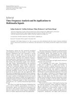
1.1 The FMCW radar transmitted (solid) and received signal frequency
(dashed). The region where the ∆f is valid is in region T . . . . . . . . 4
1.2 The Channel Input-Output Model . . . . . . . . . . . . . . . . . . . . 7

1.3 (a). Classical parametric array processing, (b). First case: PPS array
processing, (c). Second case: array processing in presence of unknown
zero-mean Gaussian noise, (d) Third case: non-parametric (blind) array
processing . . . . . . . . . . . . . . . . . . . . . . . . . . . . . . . . 9
2.1 Signal with varying frequencies over time . . . . . . . . . . . . . . . 16
2.2 Plane wave impinging from (φ
i
, ψ
i
) direction to antenna array . . . 38
2.3 Plane wave impinging from θ direction to ULA with d element interspacing 39
3.1 Comparison of MSE of f
1
(Hz)
2
vs. SNR(dB) among CBF, proposed
LS-based algorithm and CRB . . . . . . . . . . . . . . . . . . . . . . 68
3.2 Comparison of MSE of f
2
(Hz/s)
2
vs. SNR(dB) among CBF, proposed
LS-based algorithm and CRB . . . . . . . . . . . . . . . . . . . . . . 69
3.3 Comparison of MSE of θ (
o
)
2
vs. SNR(dB) among CBF, proposed LS-
based algorithm and CRB . . . . . . . . . . . . . . . . . . . . . . . . 70
3.4 Comparison of MSE of f

1
(Hz)
2
among CBF, proposed LS-based and
TLS-LS based algorithms . . . . . . . . . . . . . . . . . . . . . . . . 73
x
3.5 Comparison of MSE of f
2
(Hz/s)
2
among CBF, proposed LS-based and
TLS-LS based algorithms . . . . . . . . . . . . . . . . . . . . . . . . 74
3.6 Comparison of MSE of DOA (
o
)
2
among CBF, proposed LS-based and
TLS-LS based algorithms . . . . . . . . . . . . . . . . . . . . . . . . 75
4.1 Comparison of simulation results between the ML and the proposed
method. RMSE of f
2
(Hz/s) and DOA (
o
) as function of SNR are
in (a) and (b) respectively . . . . . . . . . . . . . . . . . . . . . . . 108
4.2 RMSE of f
2
(Hz/s) and DOA (
o
) as function of ∆ at SNR=30dB . 109

4.3 RMSE of f
3
(Hz/s
2
) and DOA (
o
) as function of SNR are in (a) and
(b), respectively . . . . . . . . . . . . . . . . . . . . . . . . . . . . . 110
5.1 TFD for one realization of example 1. The first row is TFDs of the
original sources; the second is of the mixtures at each sensor; the
third is of the estimated sources by the proposed method and the
last is of the estimated sources by existing subspace method . . . . 137
5.2 NMSE for example 2. All sources are llinear FMs . . . . . . . . . . 138
5.3 TFD for one realization of example 2. The first row is TFDs of the
original sources; the second is of the mixtures at each sensor; the
third is of the estimated sources by the proposed method and the
last is of the estimated sources by existing subspace method . . . . 139
5.4 NMSE for example 3. Sources are 3 linear FMs and one multicom-
ponent signal . . . . . . . . . . . . . . . . . . . . . . . . . . . . . . 140
5.5 TFD for one realization of example 3. The first row are TFDs of the original sources, the
second are of the mixtures at each sensor, the third are of the estimated sources by the
proposed method and the last are of the estimated sources by existing subspace method . . 141
xi
6.1 DOA estimation RMSE’s vs. SNR for two independent sources. . . 157
6.2 DOA estimation RMSE’s vs. spatial correlation coefficient of noise . 158
xii
Abbreviations
AF Ambiguity Function
BSS Blind Source Separation
CBF Chirp Beam-former

CP(s) Cross Point(s)
CRB Cramer-Rao Bound
CT(s) Cross-term(s)
DOA(s) Direction of Arrival(s)
DPT Discrete Polynomial Transform
DTFT Discrete Time Fourier Transform
Eqn(s). Equation(s)
ESPRIT Estimation of Signal Parameters via Rotational Invari-
ance Techniques
EVD Eigen-Value Decomposition
FT Fourier Transform
FFT Fast Fourier Transform
FOS Fourth-Order Statistics
xiii
FMCW Frequency Modulated Continuous Wave
HAF Higher-order Ambiguity Function
HIM Higher-order Instantaneous Moment
HO Higher-Order
HOS Higher-Order Statistics
i.i.d. Independent and Identically Distributed
JAFE Joint Angle and Frequency Estimation
LFM Linear Frequency Modulated
LS Least Squares
MAP(s) Multiple Auto Point(s)
MIMO Multiple Input Multiple Output
ML Maximum Likelihood
MMSE Minimum Mean Square Error
MSE Mean Square Error
MUSIC MUltiple SIgnal Classification
MWV Modified Wigner-Ville

NMSE Normalized Mean Square Error
pdf Probability Density Function
PPS Polynomial Phased Signal
SAP(s) Single Auto Point(s)
SAR Synthetic Aperture Radar
xiv
SAS Synthetic Aperture Sonar
SHIM Spatial Higher-order Instantaneous Moment
SIR Signal-to-Interference Ratio
SNR Signal-to-Noise Ratio
SOS Second-Order Statistics
STFD(s) Spatial Time-Frequency Distribution(s)
SVD Single Value Decomposition
TF Time-Frequency
TFD(s) Time-Frequency Distribution(s)
TLS Total Least Squares
UBSS Underdetermined Blind Source Separation
WVD Wigner-Ville Distribution
xv
Notations
(·)
T
Matrix transpose
(·)
∗
Complex conjugate
(·)
H
Hermitian transpose
(·)

−1
Generalized inverse
(·)
†
Moore-Penrose pseudo-inverse
E[·], E{·} Statistical expectation
 · ,  · 
2
2-norm
 · 
F
Frobenius norm
⊗ Kronecker product
 Khatri-Rao product, which is column-wise Kronecker product
A  B = [a
1
⊗ b
1
, a
2
⊗ b
2
, · · · ]
◦ Element-wise (Schur-Hadamard) matrix product
[A]
l,k
or (A)
l,k
The element of matrix A in row l-th and column k-th
[v]

l
or (v)
l
The l-th element of vector v
rank(A) The rank of matrix A
span(A) The column span of matrix A
tr(A), trace(A) Trace or sum of diagonal elements of matrix A
diag(v) Diagonal matrix formed by elements of vector v
xvi
diag(A) Column vector formed by diagonal elements of matrix A
vec(A) The column vector obtained from matrix A by stacking the column
vectors of A from left to right.
C
n
The set of n × 1 column vectors with complex entries
C
n×m
The set of n × m matrices with complex entries
I The identity matrix
P
A
The projection matrix onto space span(A)
{c} The real component of c
{c} The imaginary component of c
∠c The complex phase/angle of c
xvii
Chapter 1
Introduction
1.1 Background
Generally, this thesis focused on the parametric and non-parametric estimation of

signals in array systems. The parameters to be estimated include DOA and the fre-
quency parameters of signals. The most classical frequency parameter estimation
is the signal spectral estimation, which is still of interests in many applications. In
addition to that, research scope on spectral estimation has been broadened over
the last decades, not only just applying to sinusoidal signals but also applying to
wider class of signals which are more suitable in the real world settings. In the fol-
lowing subsection, we will introduce polynomial phase signals (PPS), which is the
class of signals that this thesis is focused in. Thereafter, three non-classical array
processing problems which will be studied from Chapter 2 onward are introduced.
1
CHAPTER 1. INTRODUCTION 2
1.1.1 Polynomial Phase Signals
Most of the research focused in spectral estimation of sinusoid signals. This class
of signals consists of signals with their phases being a linear function of time, or
equivalently, their (instantaneous) frequencies are constant. Estimation of the fre-
quency of this class of signals has been well investigated. A more general class of
signals consists of PPS where, as its name implies, its phase, φ(t), is a polynomial
function of time (see Eqn. (1.1)). Furthermore, this class of signals also has its fre-
quency varies as a polynomial function of time, because its angular instantaneous
frequency, φ

(t), is just the derivative of the phase with respect to time.




















s(t)  Ae
jφ(t)
φ(t) 

K
i=0
a
i
t
i
φ

(t) =
dφ(t)
dt
=

K
i=0

ia
i
t
i−1
(1.1)
A very common example in this class of signals is the linear chirp signal, where the
phase is a quadratic function of time (K = 2 in Eqn.(1.1)). Thus, the frequency
of this chirp signal is a linear function of time and hence it is also referred as LFM
signal.
Polynomial phase signals occur in natural phenomena, e.g., gravity waves [1]
and seismography. Bats’ sonar-like maneuver and their way of navigating relying
on chirp (second-order PPS) are of interest to researchers for a long time. Aside
CHAPTER 1. INTRODUCTION 3
from that, applications of chirp signals have also been reported in radar [2] and
sonar [3].
The thesis also looks into multi-component PPS signal, which is defined as
r(t) =
K

i=1
s
i
(t)
where each s
i
(t) is of the form of Eqn. (1.1) with its own set of frequency parame-
ters.
1.1.2 Radar Applications
Generally, radar can be classified as two major groups, i.e. pulse radar and FMCW
radar. A pulse radar transmits the pulse wave such that when the reflected wave

received by radar, the propagation time can be measured from the duration from
the moment the pulse is transmitted to the moment the the reflected pulse is
received. On the other hand, a FMCW radar does not transmit a short pulse signal
but transmits continuous signal. This radar changes the frequency of the sinusoid
signal linearly as a sawtooth function within a frequency band. To extract the
propagation time, the received signal, and transmitted signal are multiplied and
passed through a low pass filter. The output signal after passing through a filter
will be a single sinusoid with frequency ∆f directly proportional to the distance
from the target (see Fig. 1.1). This operation together with Fourier transform
CHAPTER 1. INTRODUCTION 4
1

Transmitted

Frequency
Received
Frequency
∆
f
f
1

f
2

∆
f

time

freq

T

Figure 1.1: The FMCW radar transmitted (solid) and received signal frequency
(dashed). The region where the ∆f is valid is in region T
(FT) for frequency analysis is actually called ambiguity function (AF); we will
generalize AF to higher-order ambiguity function (HAF) in the following chapters.
Mathematically, this AF operation in the complex form is written in the form
Af(k)  FT{s(∆n)r
∗
(∆n)} (1.2)
where s(∆n) are the samples of the current transmitted signal and r(∆n) the
samples of the reflected/received signal. The more general form of AF is defined
as
Af(γ, τ) 

x(t − τ)x
∗
(t + τ)e
−jtγ
dt (1.3)
where x(t) is the signal or data for the analysis, τ is delay parameter, and γ is a
dummy variable.
CHAPTER 1. INTRODUCTION 5
If there is only one FMCW radar operating in a certain frequency band, the
radar is capable of detecting multiple objects and estimating their relative positions
from radar. However, in the case of multiple transmitting radars operating in the
same frequency band, such as in anti-collision warning system of automobiles, each
radar will create interference burying the signal reflected from the targets. This is

critical as it could create collisions on the road.
In order to understand this vividly, suppose that there are one main radar,
one interference radar, and one object. The signals transmitted by the main radar
and the interference radar during period T are s
o
(t)  A
o
e
jω
o
t+ν
o
t
2
and s
i
(t) 
A
i
e
jω
i
t+ν
i
t
2
, respectively. Assuming also that the signal scattered by the object
to main radar is only the signal transmitted from main radar, then the noise-free
received signal by the main radar is r(t) = s
o

(t − τ) + s
i
(t), where, without loss
of generality, the delay time for s
i
(t) to reach the receiver has been ignored. The
result from the radar ambiguity function would be the FT of the following y(t),
y(t) = A
1
exp{j(2ν
o
τt + ω
o
τ − ν
o
τ
2
)} + A
2
exp{j((ω
o
− ω
i
)t + (ν
o
− ν
i
)t
2
)}

where A
1
and A
2
contain the attenuated amplitudes of A
2
o
and A
o
A
i
. The second
term of y(t) will not appear if there is no interference radar. The second term is a
chirp signal, which will bury the signal of interest if its received amplitude is large,
because the chirp component has energy spreads over the entire frequency band
of interest. Hence, suppression of this chirp component would be important. This
CHAPTER 1. INTRODUCTION 6
could be done by estimating the frequency rate and removing the second term
through filtering (advert to Chapter 3).
Another example is in the application of Doppler radar, where the relative
velocity of the object toward or away from the radar is proportional to the Doppler
frequency shift of the object. Furthermore, if the object is accelerating radially
then the radial acceleration is proportional to the Doppler frequency sweep rate,
i.e., frequency rate. Hence, estimation of frequency rate is essential to extract
the acceleration of the object. Therefore, the knowledge of initial frequencies and
frequency rates will give the knowledge of the distance of the objects from the
radar, the radial acceleration, and the radial velocity of the object. Consequently,
estimation of these parameters, or in general the parameters of PPS, would be
essential for various radar applications.
1.1.3 Array Processing

Basically, all of the problems covered by this thesis are in the area of array pro-
cessing, which can also be treated as multiple-input and multiple-output (MIMO)
problems. From practical standpoint, the setting can be interpreted as multiple-
antenna base station receiving signals from multiple users, or the antenna array of
radar receiving signals reflected from multiple targets. There are many more prob-
lems can be interpreted from this array processing setting. Figure 1.2 summarizes
the general model considered in this thesis.