Time-Domain Analysis and z Transform

CHAPTER 2
Time-Domain Analysis
and z Transform
2.1 A LINEAR, TIME-INVARIANT SYSTEM
The purpose of analysis of a discrete-time system is to find the output in either
the time or frequency domain of the system due to a discrete-time input signal. In
Chapter 1, we defined the discrete-time signal as a function of the integer variable
n, which represents discrete time, space, or some other physical variable. Given
any integer value in −∞ <n<∞, we can find the value of the signal according
to some well-defined relationship. This can be described as a mapping of the set
of integers to a set of values of the discrete-time signal. Description of this
relationship varied according to the different ways of modeling the signal. In this
chapter, we define the discrete-time system as a mapping of the set of discrete-
time signals considered as the input to the system, to another set of discrete-time
signals identified as the output of the system. This mapping can also be defined
by an analytic expression, formula, algorithm, or rule, in the sense that if we
are given an input to the system, we can find the output signal. The mapping
can therefore be described by several models for the system. The mapping or
the input–output relationship may be linear, nonlinear, time-invariant, or time-
varying. The system defined by this relationship is said to be linear if it satisfies
the following conditions.
Assume that the output is y(n) due to an input x(n) according to this rela-
tionship. If an input Kx(n) produces an output Ky(n), the system satisfies the
condition of homogeneity, where K is any arbitrary constant. Let K
1
y
1
(n) and
K
2
y

2
(n) be the outputs due to the inputs K
1
x
1
(n) and K
2
x
2
(n), respectively,
where K
1
and K
2
are arbitrary constants. If the output is K
1
y
1
(n) + K
2
y
2
(n)
when the input is K
1
y
1
(n) + K
2
y

2
(n), then the system satisfies the superposition
property. A system that satisfies both homogeneity and superposition is defined as
a linear system. If the output is y(n − M) when the input is delayed by M sam-
ples, that is, when the input is x(n − M), the system is said to be time-invariant
or shift-invariant. If the output is determined by the weighted sum of only the
previous values of the output and the weighted sum of the current and previous
Introduction to Digital Signal Processing and Filter Design, by B. A. Shenoi
Copyright © 2006 John Wiley & Sons, Inc.
32
A LINEAR, TIME-INVARIANT SYSTEM
33
values of the input, then the system is defined as a causal system. This means
that the output does not depend on the future values of the input. We will discuss
these concepts again in more detail in later sections of this chapter. In this book,
we consider only discrete-time systems that are linear and time-invariant (LTI)
systems.
Another way of defining a system in general is that it is an interconnection
of components or subsystems, where we know the input–output relationship of
these components, and that it is the way they are interconnected that determines
the input–output relationship of the whole system. The model for the DT system
can therefore be described by a circuit diagram showing the interconnection of
its components, which are the delay elements, multipliers, and adders, which are
introduced below. In the following sections we will use both of these definitions
to model discrete-time systems. Then, in the remainder of this chapter, we will
discuss several ways of analyzing the discrete-time systems in the time domain,
and in Chapter 3 we will discuss frequency-domain analysis.
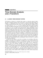
2.1.1 Models of the Discrete-Time System
First let us consider a discrete-time system as an interconnection of only three
basic components: the delay elements, multipliers, and adders. The input–output

relationships for these components and their symbols are shown in Figure 2.1.
The fourth component is the modulator, which multiplies two or more signals
and hence performs a nonlinear operation.
A simple discrete-time system is shown in Figure 2.2, where input signal
x(n) ={x(0), x(1), x(2), x(3)} is shown to the left of v
0
(n) = x(n). The signal
Delay Element
Multiplier
Adder
Modulator
m
6
(n)
X
1
(n)
Y
1
(n) = X
1
(n − 1)
Y
2
(n) = KX
2
(n)
Y
3
(n) = X

3
(n) + X
4
(n)
Y
5
(n) = X
5
(n)m
6
(n)
X
2
(n)
X
3
(n)
X
4
(n)
X
5
(n)
Σ
Σ
K
z
−1
Figure 2.1 The basic components used in a discrete-time system.
34

TIME-DOMAIN ANALYSIS AND z TRANSFORM
x(0)
x(1)
x(2)
x(3)
x(0)
x(1)
x(2)
x(3)
2
1
034
21034567
n
n
X(n)
y(n)
V
0
(n)
b(0)
b(1)
b(2)
b(3)
V
1
(n)
V
2
(n)

V
3
(n)
z
−1
z
−1
z
−1
Σ
x(0)
x(1)
x(2)
x(3)
210
3
4
56
7
n
210
x(0)
x(1)
x(2)
x(3)
34567
n
Figure 2.2 Operations in a typical discrete-time system.
v
1

(n) shown on the left is the signal x(n) delayed by T seconds or one sam-
ple, so, v
1
(n) = x(n − 1). Similarly, v(2) and v(3) are the signals obtained
from x(n) when it is delayed by 2T and 3T seconds: v
2
(n) = x(n − 2) and
v
3
(n) = x(n − 3). When we say that the signal x(n) is delayed by T,2T ,or3T
seconds, we mean that the samples of the sequence are present T,2T ,or3T
seconds later, as shown by the plots of the signals to the left of v
1
(n), v
2
(n),
and v
3
(n). But at any given time t = nT ,thesamplesinv
1
(n), v
2
(n),andv
3
(n)
are the samples of the input signal that occur T,2T ,and3T seconds previous to
t = nT . For example, at t = 3T , the value of the sample in x(n) is x(3),andthe
values present in v
1
(n), v

2
(n) and v
3
(n) are x(2), x(1),andx(0), respectively.
A good understanding of the operation of the discrete-time system as illustrated
above is essential in analyzing, testing, and debugging the operation of the sys-
tem when available software is used for the design, simulation, and hardware
implementation of the system.
It is easily seen that the output signal in Figure 2.2 is
y(n) = b(0)v(0) + b(1)v(1) + b(2)v(2) + b(3)v(3)
= b(0)x(n) + b(1)x(n − 1) + b(2)x(n − 2) + b(3)x(n − 3)
A LINEAR, TIME-INVARIANT SYSTEM
35
X(z)
ΣΣ Σ
0.8
0.5
0.3
−0.2
−0.4
0.6
−0.1
y
1
(z)
y
3
(z)
y
2

(z)
z
−1
z
−1
z
−2
y
1
(z)
z
−1
y
2
(z)
z
−1
z
−1
Figure 2.3 Schematic circuit for a discrete-time system.
where b(0), b(1), b(2), b(3) are the gain constants of the multipliers. It is also
easy to see from the last expression that the output signal is the weighted sum of
the current value and the previous three values of the input signal. So this gives
us an input–output relationship for the system shown in Figure 2.2.
Now we consider another example of a discrete-time system, shown in
Figure 2.3. Note that a fundamental rule is to express the output of the adders
and generate as many equations as the number of adders found in this circuit
diagram for the discrete-time system. (This step is similar to writing the node
equations for an analog electric circuit.) Denoting the outputs of the three adders
as y

1
(n), y
2
(n),andy
3
(n),weget
y
1
(n) = 0.3y
1
(n − 1) − 0.2y
1
(n − 2) − 0.1x(n − 1)
y
2
(n) = y
1
(n) + 0.5y
1
(n − 1) − 0.4y
2
(n − 1)
y
3
(n) = y
2
(n) + 0.6y
2
(n − 1) + 0.8y
1

(n) (2.1)
These three equations give us a mathematical model derived from the model
shown in Figure 2.3 that is schematic in nature. We can also derive (draw
the circuit realization) the model shown in Figure 2.3 from the model given in
Equations (2.1). We will soon describe a method to obtain a single input–output
relationship between the input x(n) and the output y(n) = y
3
(n), after eliminat-
ing the internal variables y
1
(n) and y
2
(n); that relationship constitutes the third
model for the system. The general form of such an input–output relationship is
y(n) =−
N

k=1
a(k)y(n − k) +
M

k=0
b(k)x(n − k) (2.2)
36
TIME-DOMAIN ANALYSIS AND z TRANSFORM
or in another equivalent form
N

k=0
a(k)y(n − k) =

M

k=0
b(k)x(n − k); a(0) = 1 (2.3)
Equation (2.2) shows that the output y(n) is determined by the weighted sum
of the previous N values of the output and the weighted sum of the current and
previous M + 1 values of the input. Very often the coefficient a(0) as shown in
(2.3) is normalized to unity.
Soon we will introduce the z transform to represent the discrete-time signals
in the set of equations above, thereby generating more models for the system, and
from these models in the z domain, we will derive the transfer function H(z
−1
)
and the unit sample response or the unit impulse response h(n) of the system.
From any one of these models in the z domain, we can derive the other models in
the z domain and also the preceding models given in the time domain. It is very
important to know how to obtain any one model from any other given model
so that the proper tools can be used efficiently, for analysis of the discrete-time
system. In this chapter we will elaborate on the different models of a discrete-
time system and then discuss many tools or techniques for finding the response of
discrete-time systems when they are excited by different kinds of input signals.
2.1.2 Recursive Algorithm
Let us consider an example of Equation (2.2) as y(n) = y(n − 1) − 0.25y(n −
2) + x(n), where the input sequence x(n) = δ(n), and the two initial conditions
are y(−1) = 1.0andy(−2) = 0.4.
We compute y(0), y(1), y(2), ... in a recursive manner as follows: y(0) =
y(−1) − 0.25y(−2) + x(0).Sincex(n) = δ(n), we substitute x(0) = 1 and get
y(0) = 1.0 − 0.25(0.4) +
1 = 1.9. Next y(1) = y(0) − 0.25y(−1) + x(1).We
know y(0) = 1.9 from the step shown above, and also that x(1) = 0. So

we get y(1) = 1.9 − 0.25(1.0) + 0 = 1.65. Next, for n = 2, when we compute
y(2) = y(1) − 0.25y(0) + x(2). Substituting the known values from above, we
get y(2) = 1.65 − 0.25(1.9) +
0 = 1.175.
Next, when n = 3, we obtain
y(3) = y(2) − 0.25y(1) + x(3)
= 1.175 − 0.25(1.65) + 0 = 0.760
We can continue to calculate the values of the output y(n) for n = 4, 5, 6, 7,....
This is known as the recursive algorithm, which we use to calculate the output
when we are given an equation of the form (2.2); it can be used when there is
any other input. For a system modeled by an equation of the form (2.2), the
output is infinite in length in general. As a special case, when the input is the
unit impulse function δ(n), and the initial conditions are assumed to be zero, the
A LINEAR, TIME-INVARIANT SYSTEM
37
resulting output is called the unit impulse response h(n) (or more appropriately
the unit sample response) and is infinite in length.
Consider a system in which the multiplier constants a(k) = 0fork =
1, 2, 3,...,N. Then Equation (2.2) reduces to the form
y(n) =
M

k=0
b(k)x(n − k) (2.4)
= b(0)x(n) + b(1)x(n − 1) + b(2)x(n − 2) +···+b(M)x(n − M)
Let us find the unit impulse response of this system, using the recursive algo-
rithm, as before:
y(0) = b(0)(1) + 0 + 0 + 0 +···=b(0)
y(1) = b(0)x(1) + b(1)x(0) + b(2)x(−1) + 0 + 0 +···=b(1)
y(2) = b(0)x(2) + b(1)x(1) + b(2)x(0) + 0 +

0 + 0 +···=b(2)
Continuing this procedure recursively, we would get
y(3) = b(3)
y(4) = b(4)
·
·
·
y(M) = b(M)
This example leads to the following two observations: (1) the samples of the unit
impulse response are the same as the coefficients b(n), and (2) therefore the unit
impulse response h(n) of the system is finite in length.
So we have shown without proof but by way of example that the unit impulse
response of the system modeled by an equation of the form (2.2) is infinite in
length, and hence such a system is known as an infinite impulse response (IIR)
filter, whereas the system modeled by an equation of the form (2.4), which has
an unit impulse response that is finite in length, is known as the finite impulse
response (FIR) filter. We will have a lot more to say about these two types of
filters later in the book. Equation (2.3) is the ordinary, linear, time-invariant,
difference equation of N th order, which, if necessary, can be rewritten in the
recursive difference equation form (2.2). The equation can be solved in the time
domain, by the following four methods:
1. The recursive algorithm as explained above
2. The convolution sum, to get the zero state response, as explained in the
next section
38
TIME-DOMAIN ANALYSIS AND z TRANSFORM
3. The classical method of solving a difference equation
4. The analytical solution using the z transform.
We should point out that methods 1–3 require that the DT system be modeled by a
single-input, single-output equation. If we are given a large number of difference

equations describing the DT system, then methods 1–3 are not suitable for finding
the output response in the time domain. Method 4, using the z transform, is the
only powerful and general method to solve such a problem, and hence it will be
treated in greater detail and illustrated by several examples in this chapter. Given
a model in the z-transform domain, we will show how to derive the recursive
algorithm and the unit impulse response h(n) so that the convolution sum can be
applied. So the z-transform method is used most often for time-domain analysis,
and the frequency-domain analysis is closely related to this method, as will be
discussed in the next chapter.
2.1.3 Convolution Sum
In the discussion above, we have assumed that the unit impulse response of a
discrete-time system when it is excited by a unit impulse function δ(n),exists
(or is known), and we denote it as h(n). Instead of using the recursive algo-
rithm to find the response due to any input, let us represent the input sig-
nal x(n) not by its values in a sequence {x(0), x(1), x(2), x(3),...} but as
the values of impulse function at the corresponding instants of time. In other
words, we consider the sequence of impulse functions x(0)δ(n), x(1)δ(n − 1),
x(2)δ(n − 2),... as the input—and not the sequence of values {x(0), x(1),
x(2), x(3),...}. The difference between the values of the samples as a sequence
of numbers and the sequence of impulse functions described above should be
clearly understood. The first operation is simple sampling operation, whereas the
second is known as impulse sampling, which is a mathematical way to repre-
sent the same data, and we represent the second sequence in a compact form:
x(n) =

∞
k=0
x(k)δ(n − k). The mathematical way of representing impulse sam-
pling is a powerful tool that is used to analyze the performance of discrete-time
systems, and the values of the impulse functions at the output are obtained by

analytical methods. These values are identified as the numerical values of the
output signal.
Since h(n) is the response due to the input δ(n),wehavex(0)h(n) as the
response due to x(0)δ(n) because we have assumed that the system is linear.
Assuming that the system is time-invariant as well as linear, we get the output
due to an input x(1)δ(n − 1) to be x(1)h(n − 1). In general, the output due to
an input x(k)δ(n − k) is given by x(k)h(n − k). Adding the responses due to all
the impulses in x(n) =

∞
k=0
x(k)δ(n − k), we get the total output as the sum
y(n) =
∞

k=0
x(k)h(n − k) (2.5)
A LINEAR, TIME-INVARIANT SYSTEM
39
This is known as the convolution sum, denoted by a compact notation y(n) =
x(n) ∗ h(n). The summation formula can be used to find the response due to any
input signal. So if we know the unit impulse response h(n) of the system, we
can find the output y(n) due to any input x(n)—therefore it is another model
for the discrete-time system. In contrast to the recursive algorithm, however,
note that the convolution sum cannot be used to find the response due to given
initial conditions. When and if the input signal is defined for −∞ <n<∞ or
−M ≤ n<∞, obviously the lower index of summation is changed to −∞.In
this case the convolution sum formula takes the general form
y(n) =
∞


k=−∞
x(k)h(n − k) (2.6)
For example, even though we know that h(n) = 0for−∞ <n<0, if the input
sequence x(n) is defined for −M<n<∞,thenwehavetousetheformula
y(n) =

∞
k=−∞
x(k)h(n − k).Ifx(n) = 0for−∞ <n<0, then we have to use
the formula y(n) =

∞
k=0
x(k)h(n − k).
To understand the procedure for implementing the summation formula, we
choose a graphical method in the following example. Remember that the recur-
sive algorithm cannot be used if the DT system is described by more than one
difference equation, and the convolution sum requires that we have the unit pulse
response of the system. We will find that these limitations are not present when
we use the z-transform method for analyzing the DT system performance in the
time domain.
Example 2.1
Given an h(n) and x(n), we change the independent variable from n to k and
plot h(k) and x(k) as shown in Figure 2.4a,b. Note that the input sequence is
defined for −2 ≤ k ≤ 5 but h(k) is a causal sequence defined for 0 ≤ k ≤ 4. Next
we do a time reversal and plot h(−k) in Figure 2.4c. When n ≥ 0, we obtain
h(n − k) by delaying (or shifting to the right) h(−k) by n samples; when n<0,
the sequence h(−k) is advanced (or shifted to the left). For every value of n,
we have h(n − k) and x(k) and we multiply the samples of h(n − k) and x(k)

at each value of k and add the products.
For our example, we show the summation of the product when n =−2in
Figure 2.4d, and show the summation of the product when n = 3inFigure2.4e.
The output y(−2) has only one nonzero product = x(−2)h(0). But the output
sample y(3) is equal to x(0)h(3) +
x(1)h(2) + x(2)h(1) + x(3)h(0).
But note that when n>9, and n<−2, the sequences h(n − k) and x(k) do
not have overlapping samples, and therefore y(n) = 0forn>9andn<−2.
Example 2.2
As another example, let us assume that the input sequence x(n) and also the
unit impulse response h(n) are given for 0 ≤ n<∞. Then output y(n) given
40
TIME-DOMAIN ANALYSIS AND z TRANSFORM
−2
−6 −5−4 −3−2 −1
−1
0
0
−4
−3 −2 −1
0
1
1
2
2
−10 1 2 3
012345 109876
3
4
5

0
1
2
3
4
k
k
k
k
k
k
X(k) h(k)
h(−2 − k)
h(− k)
h(3 − k)
h(10 − k)
(a)(b)
(d)
(c)
(e)
(f )
Figure 2.4 Convolution sum explained.
by (2.5) can be computed for each value of n as shown below:
y(0) = x(0)h(0)
y(1) = x(0)h(1) + x(1)h(0)
y(2) = x(0)h(2) + x(1)h(1) + x(2)h(0)
y(3) = x(0)h(3) + x(1)h(2) + x(2)h(1) + x(3)h(0)
y(4) = x(0)h(4) + x(1)h(3) + x(2)h(2) + x(3)h(1
) + x(4)h(0)
·

·
·
y(n) = x(0)h(n)+x(1)h(n − 1)+x(2)h(n − 2)+x(3)h(n − 3)+· · ·+x(n)h(0)
· (2.7)
·
·
z TRANSFORM THEORY
41
It is interesting to note the following pattern. In the expressions for each
value of the output y(n) above, we have x(0), x(1), x(2)... and h(n), h(n − 1),
h(n − 2)... multiplied term by term in order and the products are added, while
the indices of the two samples in each product always add to n.
Convolution is a fundamental operation carried out by digital signal processors
in hardware and in the processing of digital signals by software. The design of
digital signal processors and the software to implement the convolution sum
have been developed to provide us with very efficient and powerful tools. We
will discuss this subject again in Section 2.5, after we learn the theory and
application of z transforms.
2.2 z TRANSFORM THEORY
2.2.1 Definition
In many textbooks, the z transform of a sequence x(n) is simply defined as
Z[x(n)] = X(z) =
∞

n=−∞
x(n)z
−n
(2.8)
and the inverse z transform defined as
Z

−1
[X(z)] = x(n) =
1
2πj

C
X(z)z
n−1
dz (2.9)
Equation (2.8) represents the (double-sided or) bilateral z transform of a sequence
x(n) defined for −∞ <n<∞. The inverse z transform given in (2.9) is obtained
by an integration in the complex z plane, and this integration in the z plane is
beyond the scope of this book.
We prefer to consider signals that are of interest in digital signal processing
and hence consider a sequence obtained by sampling a continuous-time signal
x(t) with a constant sampling period T (where T is the sampling period), and
generate a sequence of numbers x(nT ). Remember that according to the sifting
theorem, we have x(t)δ(t) = x(0)δ(t). We use this result to carry out a proce-
dure called impulse sampling by multiplying x(t) with an impulse train p(t) =

∞
n=0
δ(t − nT ). Consequently we consider a sequence of delayed impulse func-
tions weighted by the strength equal to the numerical values of the signal instead
of a sequence of numbers. By doing so, we express the discrete sequence as a
function of the continuous variable t, which allows us to treat signal processing
mathematically. The product is denoted as
x
∗
(t) =

∞

n=0
x(t)δ(t − nT )
=
∞

n=0
x(nT )δ(t − nT ) (2.10)
42
TIME-DOMAIN ANALYSIS AND z TRANSFORM
This expression has a Laplace transform denoted as
X
∗
(s) =
∞

n=0
x(nT )e
−snT
(2.11)
Now we use a frequency transformation e
sT
= z, (where z is a complex variable),
and substituting it in expression (2.11), we get
X
∗
(s)



e
sT
=z
=
∞

n=0
x(nT )z
−n
Since T is a constant, we consider the samples x(nT ) as a function of n and
obtain the z transform of x(n) as
X
∗
(s)


e
sT
=z
=
∞

n=0
x(nT )z
−n
X(z) =
∞

n=0
x(n)z

−n
(2.12)
Although the first definition of a discrete sequence given in (2.8) is devoid of
any signal concepts, soon concepts such as frequency response and time-domain
response are used in the analysis of discrete-time systems and signal processing.
Our derivation of the z transform starts with a continuous-time signal that is sam-
pled by impulse sampling and introduces the transformation e
sT
= z to arrive at
the same definition. In Chapter 3, we will study the implication of this transfor-
mation in more detail and get a fundamental understanding of the relationship
between the frequency responses of the continuous-time systems and those of
the discrete-time systems. Note that we consider in this book only the unilateral
z transform as defined by (2.12), so we set the lower index in the infinite sum
as n = 0.
Example 2.3
Let us derive the z transform of a few familiar discrete-time sequences. Consider
the unit pulse
δ(n) =

1 n = 0
0 n = 0
There is only term in the z transform of δ(n), which is one when n = 0. Hence
Z
[
δ(n)
]
= 1.
z TRANSFORM THEORY
43

Example 2.4
Consider the unit sample sequence u(n)
u(n) =

1forn ≥ 0
0forn<0
(2.13)
From the definition of the z transform, we get
Z[u(n)] = 1 + z
−1
+ z
−2
+ z
−3
+··· (2.14)
=
∞

n=0
z
−n
(2.15)
This is an infinite series that converges to a closed-form expression (2.16), only
when


z
−1



< 1, or
|
z
|
> 1. This represents the region outside the unit circle in
the z plane and it is called the region of convergence (ROC). This means that
the closed-form expression exists only for values of z that lie in this region:
∞

n=0
z
−n
=
1
1 − z
−1
=
z
z − 1
(2.16)
It is obvious that the region of convergence for the z transform of δ(n) is the
entire z plane.
Example 2.5
Let x(n) = α
n
u(n),whereα is assumed to be a complex number in general.
From the definition for the z transform, we obtain
X(z) =
∞


n=0
α
n
z
−n
=
∞

n=0

αz
−1

n
(2.17)
This power series converges to (2.18), when


αz
−1


< 1, that is, when
|
z
|
>
|
α
|

.
This shows that the region of convergence for the power series is outside the
circle of radius R = α. It is important to know the region of convergence in
which the closed-form expression for the z transform of a sequence of infinite
length is valid.
1
X(z) =
1
1 − αz
−1
=
z
z − α
(2.18)
1
It can be shown that the z transform for the anticausal sequence f(n) =−α
n
u(−n − 1) is F(z) =

−1
n=−∞
α
n
z
−n
, which also converges to z/(z − α), which is the same as X(z) in (2.18), but its ROC
is
|
z
|

<α. So the inverse z transform of a function is not unique; only when we know its ROC does
the inverse z transform become unambiguous.
44
TIME-DOMAIN ANALYSIS AND z TRANSFORM
Example 2.6
Let us consider another example, x(n) = e
jθn
u(n), which is a complex-valued
sequence. Its z transform is
X(z) =
∞

n=0
e
jθn
z
−n
=
1
1 − e
jθ
z
−1
=
z
z − e
jθ
(2.19)
and its region of convergence is the region outside the unit circle in the z plane:
|

z
|
> 1.
Example 2.7
Given a sequence x(n) = r
n
cos(θn)u(n),where0<r≤ 1, to derive its z trans-
form, we express it as follows:
x(n) = r
n

e
jθn
+ e
−jθn
2

u(n)
=

r
n
e
jθn
2
+
r
n
e
−jθn

2

u(n)
=

re
jθ

n
2
u(n) +

re
−jθ

n
2
u(n) (2.20)
Now one can use the previous results and obtain the z transform of x(n) =
r
n
cos(θn)u(n) as
X(z) =
z(z − r cos(θ ))
z
2
− (2r cos(θ ))z + r
2
(2.21)
and its region of convergence is given by

|
z
|
>r. Of course, if the sequence
given is x(n) = e
−an
cos(ω
0
n)u(n), we simply substitute e
−a
for r in (2.21),
to get the z transform of x(n).Itisusefultohavealistofz transforms for
discrete-time sequences that are commonly utilized; they are listed in Table 2.1.
It is also useful to know the properties of z transforms that can be used to
generate and add more z transforms to Table 2.1, as illustrated by the following
example.
Property 2.1: Differentiation If X(z) is the z transform of x(n)u(n),
−z[dX(z)]/dz is the z transform of nx(n)u(n). We denote this property by
nx(n)u(n) ⇐⇒ − z
dX(z)
dz
(2.22)
z TRANSFORM THEORY
45
TABLE 2.1 List of z-Transform Pairs
x(n),forn ≥ 0 X(z)
1 δ(n) 1
2 δ(n − m) z
−m
3 u(n)

z
z − 1
4 au(n)
az
z − 1
5 a
n
z
z − a
6 na
n
az
(
z − a
)
2
7 n
2
z(z + 1)
(z − 1)
3
8 n
3
z(z
2
+ 4z + 1)
(z − 1)
4
9 n
2

a
n
az(z + a)
(z − a)
3
10
n(n − 1)
2!
a
n−2
z
(z − a)
3
11
n(n − 1)(n − 2) ·······(n − m + 2)
(m − 1)!
a
n−m+1
z
(z − a)
m
12 r
n
e
jθn
z
z − re
jθ
13 r
n

cos(θn)
z(z − r cos(θ))
z
2
− (2r cos(θ ))z + r
2
14 r
n
sin(θn)
rzsin(θ )
z
2
− (2r cos(θ ))z + r
2
15 e
−αn
cos(θn)
z(z − e
−α
cos(θ))
z
2
− (2e
−α
cos(θ))z + e
−2α
Proof : X(z) =

∞
n=0

x(n)z
−n
. Differentiating both sides with respect to z,
we get
dX(z)
dz
=
∞

n=0
x(n)

−nz
−n−1

=−z
−1
∞

n=0
nx(n)z
−n
−z
dX(z)
dz
=
∞

n=0
nx(n)z

−n
= Z[nx(n)u(n)]
46
TIME-DOMAIN ANALYSIS AND z TRANSFORM
Now consider the z transform given by (2.18) and also listed in Table 2.1:
x(n) = a
n
u(n) ⇐⇒
z
z − a
= X(z) (2.23)
Using this differentiation property recursively, we can show that
na
n
u(n) ⇐⇒
az
(z − a)
2
(2.24)
and
n
2
a
n
u(n) ⇐⇒
az(z + a)
(z − a)
3
(2.25)
From these results, we can find the z transform of

1
2
(n + 1)(n + 2)a
n
u(n) =
1
2
(n
2
+ 3n + 2)a
n
u(n) as follows:
1
2
(n + 1)(n + 2)a
n
u(n) ⇐⇒
z
3
(z − a)
3
(2.26)
The transform pair given by (2.26) is an addition to Table 2.1. Indeed, we can
find the z transforms of n
3
a
n
u(n), n
4
a

n
u(n),..., using (2.22) and then find the
z transforms of
1
3!
(n + 1)(n + 2)(n + 3)a
n
u(n)
1
4!
(n + 1)(n + 2)(n + 3)(n + 4)a
n
u(n) (2.27)
·
·
·
which can be added to Table 2.1.
Properties of z transform are useful for deriving the z transform of new
sequences. Also they are essential for solving the linear difference equations and
finding the response of discrete-time systems when the input function and initial
conditions are given. Instead of deriving all the properties one after another, as is
done in many textbooks, we derive one or two at a time and immediately show
their applications.
Property 2.2: Delay Let the z transform of x(n)u(n) be X(z) =

∞
n=0
x(n)z
−n
=

x(0) + x(1)z
−1
+ x(2)z
−2
+ x(3)z
−3
+···.
Then the z transform of x(n − 1)u(n − 1) is z
−1
X(z) + x(−1):
x(n − 1)u(n − 1) ⇐⇒ z
−1
X(z) + x(−1) (2.28)
z TRANSFORM THEORY
47
Proof :Thez transform of x(n − 1)u(n − 1) is obtained by shifting to the
right or delaying x(n)u(n) by one sample, and if there is a sample x(−1) at
n =−1, it will be shifted to the position n = 0. The z transform of this delayed
sequence is therefore given by
x(−1) + x(0)z
−1
+ x(1)z
−2
+ x(2)z
−3
+···
= x(−1) + z
−1

x(0) + x(1)z

−1
+ x(2)z
−2
+···

= x(−1) + z
−1
X(z)
By repeated application of this property, we derive
x(n − 2)u(n − 2) ⇐⇒ z
−2
X(z) + z
−1
x(−1) + x(−2) (2.29)
x(n − 3)u(n − 3) ⇐⇒ z
−3
X(z) + z
−2
x(−1) + z
−1
x(−2) + x(−3) (2.30)
and
x(n − m)u(n − m) ⇐⇒ z
−m
X(z
−1
) + z
−m+1
x(−1) + z
−m+2

x(−2)
+···+x(−m)
or
x(n − m)u(n − m) ⇐⇒ z
−m
X(z) +
m−1

n=0
x(n − m)z
−n
(2.31)
If the initial conditions are zero, we have the simpler relationship
x(n − m)u(n − m) ⇐⇒ z
−m
X(z) (2.32)
Example 2.8
Let us consider an example of solving a first-order linear difference equation
using the results obtained above. We have
y(n) − 0.5y(n − 1) = 5x(n − 1) (2.33)
where
x(n) = (0.2)
n
u(n)
y(−1) = 2
Let Z[y(n)] = Y(z). From (2.28), we have Z[y(n − 1)] = z
−1
Y(z)+ y(−1)
and Z[x(n − 1)] = z
−1

X(z) + x(−1) where X(z) = z/(z − 0.2) and x(−1) = 0,
since x(n) is zero for −∞ <n<0. Substituting these results, we get
Y(z)− 0.5

z
−1
Y(z)+ y(−1)

= 5

z
−1
X(z) + x(−1)

Y(z)− 0.5

z
−1
Y(z)+ y(−1)

= 5z
−1
X(z)
48
TIME-DOMAIN ANALYSIS AND z TRANSFORM
Y(z)

1 − 0.5z
−1


= 0.5y(−1) + 5z
−1
X(z) (2.34)
Y(z) =
0.5y(−1)
(1 − 0.5z
−1
)
+
5z
−1
(1 − 0.5z
−1
)
X(z)
Y(z) =
0.5y(−1)z
(z − 0.5)
+
5
(z − 0.5)
X(z)
Substituting y(−1) = 2andX(z) = z/(z − 0.2) in this last expression, we get
Y(z) =
z
(z − 0.5)
+
5z
(z − 0.5)(z − 0.2)
(2.35)

= Y
0i
(z) + Y
0s
(z) (2.36)
where Y
0i
(z) is the z transform of the zero input response and Y
0s
(z) is the
z transform of the zero state response as explained below.
Nowwehavetofindtheinversez transform of the two terms on the right
side of (2.35). The inverse transform of the first term Y
0i
(z) = z/(z − 0.5) is
easily found as y
0i
(n) = (0.5)
n
u(n). Instead of finding the inverse z transform
of the second term by using the complex integral given in (2.9), we resort to
the same approach as used in solving differential equations by means of Laplace
transform, namely, by decomposing Y
0s
(z) into its partial fraction form to obtain
the inverse z transform of each term. We have already derived the z transform of
Ra
n
u(n) as Rz/(z − a), and it is easy to write the inverse z transform of terms
like R

k
z/(z − a
k
). Hence we should expand the second term in the form
Y
0s
(z) =
R
1
z
z − 0.5
+
R
2
z
z − 0.2
(2.37)
by a slight modification to the partial fraction expansion procedure that we are
familiar with. Dividing Y
0s
(z) by z,weget
Y
0s
(z)
z
=
5
(z − 0.5)(z − 0.2)
=
R

1
z − 0.5
+
R
2
z − 0.2
Now we can easily find the residues R
1
and R
2
using the normal procedure and
get
R
1
=
Y
0s
(z)
z
(z − 0.5)




z=0.5
=
5
(z − 0.2)





z=0.5
= 16.666
R
2
=
Y
0s
(z)
z
(z − 0.2)




z=0.2
=
5
(z − 0.5)




z=0.2
=−16.666
Therefore
Y
0s
(z)

z
=
5
(z − 0.5)(z − 0.2)
=
16.666
z − 0.5
−
16.666
z − 0.2
z TRANSFORM THEORY
49
Multiplying both sides by z,weget
Y
0s
(z) =
16.666z
z − 0.5
−
16.666z
z − 0.2
(2.38)
Now we obtain the inverse z transform y
0s
(n) = 16.666[(0.5)
n
− (0.2)
n
]u(n).
The total output satisfying the given difference equation is therefore given as

y(n) = y
0i
(n) + y
0s
(n) =

(0.5)
n
+ 16.666[(0.5)
n
− (0.2)
n
]

u(n)
=

17.6666(0.5)
n
− 16.666(0.2)
n

u(n)
Thus the modified partial fraction procedure to find the inverse z transform of
any function F(z) is to divide the function F(z) by z, expand F(z)/z into its
normal partial fraction form, and then multiply each of the terms by z to get
F(z) in the form

k=1
R

k
z/(z − a
k
). From this form, the inverse z transform
f(n) is obtained as

k=1
R
k
(a
k
)
n
u(n).
However, there is an alternative method, to expand a transfer function expressed
in the form, when it has only simple poles
H(z
−1
) =
N(z
−1
)

k=1
(1 − a
k
z
−1
)
to its partial fraction form

H(z
−1
) =

k=1
R
k
(1 − a
k
z
−1
)
(2.39)
where
R
k
= H(z
−1
)(1 − a
k
z
−1
)


z=a
k
Then the inverse z transform is the sum of the inverse z transform of all the terms
in (2.39): h(n) =


K
k=1
R
k
(a
k
)
n
u(n). We prefer the first method because we are
already familiar with the partial fraction expansion of H(s) and know how to
find the residues when it has multiple poles in the s plane. This method will be
illustrated by several examples that are worked out in the following pages.
2.2.2 Zero Input and Zero State Response
In Section 2.2.1, the total output y(n) was obtained as the sum of two outputs
y
0i
(n) = (0.5)
n
u(n) and y
0s
(n) = 16.666[(0.5)
n
− (0.2)
n
]u(n).
If the input function x(n) is zero, then X(z) = 0, and Y(s) in (2.34) will
contain only the term Y
0i
(z) = 0.5y(−1)z/(z − 0.5) = z/(z − 0.5); therefore the
response y(n) = (0.5)

n
u(n) when the input is zero. The response of a system
described by a linear difference equation, when the input to the system is assumed
50
TIME-DOMAIN ANALYSIS AND z TRANSFORM
to be zero is called the zero input response and is determined only by the initial
conditions given. The initial conditions specified with the difference equation are
better known as initial states.(Butthetermstate has a specific definition in the
theory of linear discrete-time systems, and the terminology of initial states is con-
sistent with this definition.) When the initial state y(−1) in the problem presented
above is assumed to be zero, the z transform of the total response Y(z) contains
only the term Y
0s
(z) = 5/(z − 0.5)X(z) = 5/[(z − 0.5)(z − 0.2)], which gives a
response y
0s
(n) = 16.666[(0.5)
n
− (0.2)
n
]u(n). This is the response y(n) when
the initial condition or the initial state is zero and hence is called the zero state
response. The zero state response is the response due to input only, and the zero
input response is due to the initial states (initial conditions) only. We repeat it
in order to avoid the common confusion that occurs among students! The zero
input response is computed by neglecting the input function and computing the
response due to initial states only, and the zero state response is computed by
neglecting the initial states (if they are given) and computing the response due to
input function only. Students are advised to know the exact definition and mean-
ing of the zero input response and zero state response, without any confusion

between these two terms.
2.2.3 Linearity of the System
If the input x(n) to the discrete-time system described by (2.33) is multiplied
by a constant, say, K = 10, the total response of the system y(n) is given as
y
0i
(n) + 10y
0s
(n), which is not 10 times the total response y
0i
(n) + y
0s
(n).This
may give rise to the incorrect inference that the system described by the difference
equation (2.33) above, is not linear. The correct way to test whether a system
is linear is to apply the test on the zero state response only or to the zero input
response only as explained below.
Let the zero state response of a system defined by a difference equation be
y
1
(n) when the input to the system is x
1
(n) and the zero state response be y
2
(n)
when the input is x
2
(n), where the inputs are arbitrary. Here we emphasize that
the definition should be applied to the zero state response only or to the zero input
only. So the definition of a linear system given in Section 2.1 is repeated below,

emphasizing that the definition should be applied to the zero input response or
zero state response only.
Given a system x(n) ⇒ y(n),ifKx(n) ⇒ Ky(n) and K
1
x
1
(n) + K
2
x
2
(n) ⇒
K
1
y
1
(n) + K
2
y
2
(n), then the system is linear, provided y(n) is the zero state
response due to an input signal x(n) or the zero input response due to initial
states. Now it should be easy to verify that the system described by (2.33) is a
linear system.
2.2.4 Time-Invariant System
Let a discrete-time system be defined by a linear difference equation of the
general form (2.3), which defines the input–output relationship of the system.
USING z TRANSFORM TO SOLVE DIFFERENCE EQUATIONS
51
Let us denote the solution to this equation as the output y(n) when an input x(n)
is applied. Such a system is said to be time-invariant if the output is y(n − N)

when the input is x(n − N), which means that if the input sequence is delayed
by N samples, the output also is delayed by N samples. For this reason, a time-
invariant discrete-time system is also called a shift-invariant system. Again from
the preceding discussion about linearity of a system, it should be obvious the
output y(n) and y(n − N) must be chosen as the zero state response only or
the zero input response only, when the abovementioned test for a system to be
time-invariant is applied.
2.3 USING z TRANSFORM TO SOLVE DIFFERENCE EQUATIONS
We will consider a few more examples to show how to solve a linear shift-
invariant difference equation, using the z transform in this section, and later we
show how to solve a single-input, single-output difference equation using the
classical method. Students should be familiar with the procedure for decompos-
ing a proper, rational function of a complex variable in its partial fraction form,
when the function has simple poles, multiple poles, and pairs of complex conju-
gate poles. A “rational” function in a complex variable is the ratio between two
polynomials with real coefficients, and a “proper” function is one in which the
degree of the numerator polynomial is less than that of the denominator polyno-
mial. It can be shown that the degree of the numerator in the transfer function
H(s) of a continuous-time system is at most equal to that of its denominator. In
contrast, it is relevant to point out that the transfer function of a discrete-time
system when expressed in terms of the variable z
−1
need not be a proper func-
tion. For example, let us consider the following example of an improper function
of the complex variable z
−1
:
H(z
−1
) =

z
−4
− 0.8z
−3
− 2.2z
−2
− 0.4z
−1
z
−2
− z
−1
+ 2.0
(2.40)
In this equation, the coefficients of the two polynomials are arranged in descend-
ing powers of z
−1
, and when we carry out a long division of the numerator by
the denominator, until the remainder is a polynomial of a degree lower than that
in the denominator, we get the quotient (z
−2
+ 0.2z
−1
− 4.0) and a remainder
(−4.8z
−1
+ 8.0):
H(z
−1
) = z

−2
+ 0.2z
−1
− 4.0 +
−4.8z
−1
+ 8.0
z
−2
− z
−1
+ 2.0
(2.41)
= z
−2
+ 0.2z
−1
− 4.0 + H
1
(z
−1
) (2.42)
Since the inverse z transform of z
−m
is δ(n − m),wegettheinversez trans-
form of the first three terms as δ(n − 2) + 0.2δ(n − 1) − 4.0δ(n),andweaddit
to the inverse z transform of the H
1
(z
−1

), which will be derived below.
52
TIME-DOMAIN ANALYSIS AND z TRANSFORM
Example 2.9: Complex Conjugate Poles
Let us choose the second term on the right side of (2.41) as an example of a
transfer function with complex poles:
H
1
(z
−1
) =
−4.8z
−1
+ 8.0
z
−2
− z
−1
+ 2.0
Multiplying the numerator and denominator by z
2
, and factorizing the denomina-
tor, we find that H
1
(z
−1
) has a complex conjugate pair of poles at 0.25 ± j 0.6614:
H
1
(z) =

8(z
2
− 0.6z)
2z
2
− z + 1
=
8(z
2
− 0.6z)
2(z
2
− 0.5z + 0.5)
= 4
(z
2
− 0.6z)
(z − 0.25 − j 0.6614)(z − 0.25 + j 06614)
Let us expand H
1
(z)/z into its modified partial fraction form:
H
1
(z)
z
=
2 + j 1.0583
z − 0.25 − j 0.6614
+
2 − j 1.0583

z − 0.25 + j 0.6614
.
It is preferable to express the residues and the poles in their exponential form
and then multiply by z to get
H
1
(z) =

2.2627e
j0.4867

z
z − 0.7071e
j1.209
+

2.2627e
−j0.4867

z
z − 0.7071e
−j1.209
The inverse z transform of H
1
(z) is given by
h
1
(n) =

2.2627e

j0.4867

(0.7071e
j1.209
)
n
+

2.2627e
−j0.4867

(0.7071e
−j1.209
)
n

u(n)
=

2.2627(0.7071)
n
e
j1.209n
e
j0.4867
+ 2.2627(0.7071)
n
e
−j1.209n
e

−j0.4867

u(n)
= 2.2627(0.7071)
n

e
j(1.209n+0.4867)
+ e
−j(1.209n+0.4867)

u(n)
= 2.2627(0.7071)
n
{
2cos(1.209n + 0.4867)
}
u(n)
= 4.5254(0.7071)
n
{
cos(1.209n + 0.4867)
}
u(n).
Adding these terms, we get the inverse z transform of
H(z
−1
) = z
−2
+ 0.2z

−1
− 4.0 +

2.2627e
j0.4867

z
z − 0.7071e
j1.209
+

2.2627e
−j0.4867

z
z − 0.7071e
−j1.209
USING z TRANSFORM TO SOLVE DIFFERENCE EQUATIONS
53
h(n) = δ(n − 2) + 0.2δ(n − 1) − 4.0δ(n) + 2.2627e
j0.4867
(0.7071e
j1.209
)
n
+ 2.2627e
j −0.4867
(0.7071e
−j1.209
)

n
u(n)
= δ(n − 2) + 0.2δ(n − 1) − 4.0δ(n) + 2.2627(0.7071)
n
×{e
j(1.209n+0.4867)
+ e
−j(1.209n+0.4867)
}u(n)
= δ(n − 2) + 0.2δ(n − 1) − 4.0δ(n) + 2.2627(0.7071)
n
×{2cos(1.209n + 0.4867)}u(n)
= δ(n − 2) + 0.2δ(n − 1) − 4.0δ(n)
+ 4.5254(0.7071)
n
{
cos(1.209n + 0.4867)
}
u(n)
Note that the angles in this solution are expressed in radians.
Example 2.10
Let us consider a discrete-time system described by the linear shift-invariant
difference equation of second order given below
y(n) = 0.3y(n − 1) − 0.02y(n − 2) + x(n) − 0.1x(n − 1)
where
x(n) = (−0.2)
n
u(n)
y(−1) = 1.0
y(−2) = 0.6

Using the z transform for each term in this difference equation, we get
Y(z) = 0.3[z
−1
Y(z)+ y(−1)] − 0.02[z
−2
Y(z)+ z
−1
y(−1) + y(−2)]
+ X(z) − 0.1[z
−1
X(z) + x(−1)]
We know X(z) = z/(z + 0.2) and x(−1) = 0. Substituting these and the given
initial states, we get
Y(z)[1 − 0.3z
−1
+ 0.02z
−2
] = [0.3y(−1) − 0.02z
−1
y(−1) − 0.02y(−2)]
+ X(z)[1 − 0.1z
−1
]
Y(z) =
[0.3y(−1) − 0.02z
−1
y(−1) − 0.02y(−2)]
[1 − 0.3z
−1
+ 0.02z

−2
]
+
X(z)[1 − 0.1z
−1
]
[1 − 0.3z
−1
+ 0.02z
−2
]
54
TIME-DOMAIN ANALYSIS AND z TRANSFORM
When the input x(n) is zero, X(z) = 0; hence the second term on the right side
is zero, leaving only the first term due to initial conditions given. It is the z
transform of the zero input response y
0i
(n).
The inverse z transform of this first term on the right side
Y
0i
(z) =
[0.3y(−1) − 0.02z
−1
y(−1) − 0.02y(−2)]
[1 − 0.3z
−1
+ 0.02z
−2
]

gives the response when the input is zero, and so it is the zero input response
y
0i
(n). The inverse z transform of
X(z)[1 − 0.1z
−1
]
[1 − 0.3z
−1
+ 0.02z
−2
]
= Y
0s
(z)
gives the response when the initial conditions (also called the initial states) are
zero, and hence it is the zero state response y
0s
(n).
Substituting the values of the initial states and for X(z), we obtain
Y
0i
(z) =
[0.288 − 0.02z
−1
]
[1 − 0.3z
−1
+ 0.02z
−2

]
=
[0.288z
2
− 0.02z]
z
2
− 0.3z + 0.02
=
z[0.288z − 0.02]
(z − 0.1)(z − 0.2)
and
Y
0s
(z) =
X(z)[1 − 0.1z
−1
]
[1 − 0.3z
−1
+ 0.02z
−2
]
=

z
z + 0.2

[1 − 0.1z
−1

]
[1 − 0.3z
−1
+ 0.02z
−2
]
=
z[z
2
− 0.1z]
(z + 0.2)(z
2
− 0.3z + 0.02)
=
z
2
(z − 0.1)
(z + 0.2)(z − 0.1)(z − 0.2)
We notice that there is a pole and a zero at z = 0.1 in the second term on the
right, which cancel each other, and Y
0s
(z) reduces to z
2
/[(z + 0.2)(z − 0.2)]. We
divide Y
0i
(z) by z, expand it into its normal partial fraction form
Y
0i
(z)

z
=
[0.288z − 0.02]
(z − 0.1)(z − 0.2)
=
0.376
(z − 0.2)
−
0.088
(z − 0.1)
and multiply by z to get
Y
0i
(z) =
0.376z
(z − 0.2)
−
0.088z
(z − 0.1)
Similarly, we expand Y
0s
(z)/z = z/[(z + 0.2)(z − 0.2)] in the form −0.5/(z +
0.2) + 0.5/(z − 0.2) and get
Y
0s
(z) =
z
2
(z + 0.2)(z − 0.2)
=

−0.5z
(z + 0.2)
+
0.5z
(z − 0.2)
Therefore, the zero input response is y
0i
(n) = [0.376(0.2)
n
− 0.088(0.1)
n
]u(n)
and the zero state response is y
0s
(n) = 0.5[−(−0.2)
n
+ (0.2)
n
]u(n).
USING z TRANSFORM TO SOLVE DIFFERENCE EQUATIONS
55
Example 2.11: Multiple Poles
Here we discuss the case of a function that has multiple poles and expand it into
its partial fraction form. Let
G(z)
z
=
N(z)
(z − z
0

)
r
(z − z
1
)(z − z
2
)(z − z
3
) ···(z − z
m
)
Its normal partial fraction is in the form
G(z)
z
=
C
0
(z − z
0
)
r
+
C
1
(z − z
0
)
r−1
+···+
C

r−1
(z − z
0
)
+
k
1
(z − z
1
)
+
k
2
(z − z
2
)
+···+
k
m
(z − z
m
)
The residues k
1
,k
2
,...,k
m
for the simple poles at z
1

,z
2
,... are obtained by
the normal method of multiplying G(z)/z by (z − z
i
), i = 1, 2, 3,...,m and
evaluating the product at z = z
i
. The residue C
0
is also found by the same
method:
C
0
=

(z − z
0
)
r
G(z)
z





z=z
0
The coefficient C

1
is found from
d
dz

(z − z
0
)
r
G(z)
z





z=z
0
and the coefficient C
2
is found from
1
2
d
2
dz
2

(z − z
0

)
r
G(z)
z





z=z
0
The general formula for finding the coefficients C
j
, j = 1, 2, 3,...,(r − 1) is
C
j
=
1
j!
d
j
dz
j

(z − z
0
)
r
G(z)
z






z=z
0
(2.43)
After obtaining the residues and the coefficients, we multiply the expansion by z:
G(z) =
C
0
z
(z − z
0
)
r
+
C
1
z
(z − z
0
)
r−1
+···+
C
r−1
z
(z − z

0
)
+
k
1
z
(z − z
1
)
+
k
2
z
(z − z
2
)
+···+
k
m
z
(z − z
m
)
Then we find the inverse z transform of each term to get g(n),usingthez
transform pairs given in Table 2.1. To illustrate this method, we consider the
56
TIME-DOMAIN ANALYSIS AND z TRANSFORM
function G(z), which has a simple pole at z = 1 and a triple pole at z = 2:
G(z) =
z(2z

2
− 11z + 12)
(z − 1)(z − 2)
3
(2.44)
G(z)
z
=
(2z
2
− 11z + 12)
(z − 1)(z − 2)
3
=
C
0
(z − 2)
3
+
C
1
(z − 2)
2
+
C
2
(z − 2)
+
k
(z − 1)

k =
(2z
2
− 11z + 12)
(z − 2)
3




z=1
=−3
C
0
=
(2z
2
− 11z + 12)
(z − 1)




z=2
=−2
C
1
=
d
dz


(2z
2
− 11z + 12)
(z − 1)





z=2
=

2z
2
− 4z − 1
(z − 1)
2





z=2
=−1
C
2
=
1
2

d
2
dz
2

(2z
2
− 11z + 12)
(z − 1)





z=2
=
1
2
d
dz

2z
2
− 4z − 1
(z − 1)
2






z=2
= 3
Therefore we have
G(z) =
−2z
(z − 2)
3
+
−z
(z − 2)
2
+
3z
(z − 2)
+
−3z
(z − 1)
(2.45)
Now note that the inverse z transform of az/(z − a)
2
is easily obtained from
Table 2.1, as na
n
u(n). We now have to reduce the term −z/(z − 2)
2
to −(
1
2
)2z/

(z − 2)
2
so that its inverse z transform is correctly written as −(
1
2
)n2
n
u(n).From
the transform pair 6 in Table 2.1, we get the inverse z transform of z/(z − a)
3
as n(n − 1)/2!a
n−2
u(n).
Therefore the inverse z transform of −2z/(z − 2)
3
is obtained as
−2n(n − 1)
2!
(2)
n−2
u(n) =
−n(n − 1)
4
(2)
n
u(n)
Finally, we get the inverse z transform of G(z) as

−n(n − 1)
4

(2)
n
−
n
2
(2)
n
− 3(2)
n
− 3

u(n)
2.3.1 More Applications of z Transform
In this section, we consider the circuit shown in Figure 2.5 and model it by
equations in the z domain, instead of the equivalent model given by equations
(2.1) in the time domain. This example is chosen to illustrate the analysis of a
discrete-time system that has a large number of adders and hence gives rise to
a large number of difference equations in the z domain. Writing the z transform