Intelligent control of mechatronic systems

Adaptive Neural Network Control and its
Applications
Pey Yuen Tao
B. Eng (Hons.), The National University of Singapore
A THESIS SUBMITTED
FOR THE DEGREE OF DOCTOR OF PHILOSOPHY
NUS GRADUATE SCHOOL FOR INTEGRATIVE SCIENCES &
ENGINEERING
NATIONAL UNIVERSITY OF SINGAPORE
2008
Acknowledgments
First of all, to my thesis supervisor, Professor Shuzhi Sam Ge, for all the learning
opportunities, his unwavering support, inspiring guidance, and for his time and effort
that he has spent on my training and education. I would like to thank Dr Wei Lin and Dr
Xiaoqi Chen, my current and former thesis co-supervisors, for their guidance and help
on all matters concerning my research. I would also like to thank Professor Jianxin Xu,
for his insightful advice and guidance.
To fellow co-workers and friends in the Mechatronics and Automation Lab, and the
Edutainment Robotics Lab. Special thanks to Dr Cheng Heng Fua and Mr Keng Peng
Tee, for the interesting discussions and time we spent working together. To the TechX
team, in particular, Mr Aswin Thomas Abraham, Mr Brice Rebsamen, Mr Chenguang
Yang, Ms Bahareh Ghotbi, Mr Dong Huang, Mr Hooman Samani, Dr Qinghua Xia
and many others that have been part of the team, for the stressful but exciting time
we have spent developing and testing the system. To Professor Hongbin Du from East
China University of Science and Technology, Professor Tianping Zhang from Yangzhou
University and Professor Zhijun Li from Shanghai Jiao Tong University, for the many
enlightening discussions and help they have provided in my research. To Dr Feng Guan,
Dr Xuecheng Lai, Dr Zhuping Wang, Mr Voon Ee How, Mr Sie Chyuan Lau, Ms Beibei
Ren, Ms Yaozhang Pan, and many more, for their friendship and help.
To my family and close friends for their support and encouragement. They have
always been there for me, stood by me through the good times and the bad.

Finally, I am very grateful to the Agency of Science, Technology and Research
(A*STAR) and the NUS Graduate School of Integrative Sciences and Engineering
(NGS), for their funding and support.
ii
Abstract
This thesis considers the theoretical aspects of adaptive neural network (NN) con-
trol and its applications. Traditional adaptive controls are limited to systems where the
dynamics can be expressed in the linear-in-parameters form, while NNs can approx-
imate, to an arbitrary degree of accuracy, any real continuous function on a compact
set. Through exploiting the approximation capabilities of the NNs, a NN based control
can be developed where NNs are used to compensate for the functional and parametric
uncertainties in the system model.
In this thesis, the focus is on the control problem of a class of uncertain nonlin-
ear pure-feedback single-input single-output (SISO) systems. The non-affine nonlinear
control problem is challenging due to the relatively fewer mathematical tools available
in comparison with that for affine nonlinear systems. In particular, it is difficult to
construct control laws because pure-feedback systems have no affine appearance of the
variables which can be used as virtual controls. In this thesis, an Adaptive Variable
Structure Control (AVSC) is proposed, based on NN parametrization, for the class of
uncertain nonlinear pure-feedback single-input single-output (SISO) systems.
For the design of the AVSC, three backstepping approaches are explored in this
thesis where the comparative advantages are highlighted during the design stages and
based on the simulation studies. First, decoupled backstepping is proposed due to the
possibility of a circular control design if traditional backstepping methods are used
to cancel the coupled terms since the virtual control coefficients are still non-affine.
Subsequently, a coupled backstepping approach is adopted where the coupled terms are
handled in the next step in order to remove an assumption made on the system that was
required in decoupled backstepping. Finally, the design of the AVSC with dynamic
iii
surface control (DSC) is explored to further reduce the size of the NNs required.

In the subsequent chapter, the application of intelligent control is studied, where the
focus is on the control of marine shafting systems. A case study on the application of in-
telligent control in marine shafting systems modeled as a chained multiple mass-spring
system is presented where the control objectives include the tracking of the desired tra-
jectory and the reduction of torsional vibrations within the shafting system. In the ap-
plication study, the control design is closely coupled with the system model. Therefore,
the system model for the marine shafting system is first presented where the system
model contains functional and parametric uncertainties. The functional uncertainties
include the hydrodynamic forces acting on the propeller, which are highly nonlinear
and subjected to variations due to the diverse operating conditions such as air suction,
cavitation and partial/full emergence of the propellers, and the frictional forces acting
on the shafting system. The parametric uncertainties include the unknown moment of
inertia of each mass unit and torsional stiffness of the massless springs connecting the
mass units.
Considering the dynamic model of the system and the uncertainties, an adaptive NN
control is proposed where NNs are used to approximate the functional and parametric
uncertainties in the system. In this application study, two adaptive NN controls are de-
veloped for the marine shafting system, where the first control is uses the decoupled
backstepping approach followed by a second control design where the DSC approach
is adopted. A simulation study is conducted to illustrate the effects of the two pro-
posed controls and to analyze the difference in the two approaches in particular on the
implementation and performance issues.
iv
Contents
Acknowledgments ii
Abstract iii
Table of Contents vi
List of Figures vi
1 Introduction 1
1.1 Adaptive Variable Structure Control . . . . . . . . . . . . . . . . . . . 2

1.2 Adaptive NN Control of Marine Shafting System . . . . . . . . . . . . 6
1.3 Thesis Outline . . . . . . . . . . . . . . . . . . . . . . . . . . . . . . . 8
2 AVSC with Decoupled Backstepping 10
2.1 Introduction . . . . . . . . . . . . . . . . . . . . . . . . . . . . . . . . 10
2.2 Problem Formulation and Preliminaries . . . . . . . . . . . . . . . . . 11
2.3 Neural Networks and Parametrization . . . . . . . . . . . . . . . . . . 15
2.4 Control Design . . . . . . . . . . . . . . . . . . . . . . . . . . . . . . 17
2.5 Stability Analysis . . . . . . . . . . . . . . . . . . . . . . . . . . . . . 27
2.6 Simulation . . . . . . . . . . . . . . . . . . . . . . . . . . . . . . . . . 34
3 AVSC with Coupled Backstepping 45
3.1 Introduction . . . . . . . . . . . . . . . . . . . . . . . . . . . . . . . . 45
3.2 Problem Formulation and Preliminaries . . . . . . . . . . . . . . . . . 46
3.3 Control Design . . . . . . . . . . . . . . . . . . . . . . . . . . . . . . 47
3.4 Stability Analysis . . . . . . . . . . . . . . . . . . . . . . . . . . . . . 53
3.5 Simulation . . . . . . . . . . . . . . . . . . . . . . . . . . . . . . . . . 55
4 AVSC with Dynamic Surface Control 71
4.1 Introduction . . . . . . . . . . . . . . . . . . . . . . . . . . . . . . . . 71
4.2 Problem Formulation and Preliminaries . . . . . . . . . . . . . . . . . 72
4.3 Neural Networks for Dynamic Surface Control . . . . . . . . . . . . . 73
4.4 Control Design . . . . . . . . . . . . . . . . . . . . . . . . . . . . . . 74
4.5 Stability Analysis . . . . . . . . . . . . . . . . . . . . . . . . . . . . . 87
4.6 Simulation . . . . . . . . . . . . . . . . . . . . . . . . . . . . . . . . . 91
v
Contents
5 Adaptive NN Control of Marine Shafting System 106
5.1 Introduction . . . . . . . . . . . . . . . . . . . . . . . . . . . . . . . . 106
5.2 Dynamic Modeling . . . . . . . . . . . . . . . . . . . . . . . . . . . . 107
5.3 Adaptive NN Control with Decoupled Backstepping . . . . . . . . . . 108
5.4 Adaptive NN Control with DSC . . . . . . . . . . . . . . . . . . . . . 119
5.5 Simulation . . . . . . . . . . . . . . . . . . . . . . . . . . . . . . . . . 134

5.5.1 Adaptive NN Control with Decoupled Backstepping . . . . . . 135
5.5.2 Adaptive NN Control with DSC . . . . . . . . . . . . . . . . . 139
6 Conclusion and Future Work 145
6.1 Summary and Contributions . . . . . . . . . . . . . . . . . . . . . . . 145
6.1.1 Adaptive Variable Structure Control . . . . . . . . . . . . . . . 146
6.1.2 Adaptive NN Control of Marine Shafting System . . . . . . . . 147
6.2 Future Work . . . . . . . . . . . . . . . . . . . . . . . . . . . . . . . . 148
Bibliography 149
A Derivations for Simulation 157
B Author’s Publications 165
vi
List of Figures
2.1 Neural network compact sets . . . . . . . . . . . . . . . . . . . . . . . 33
2.2 State variables x
1
, x
2
, and x
3
under AVSC with decoupled backstepping 38
2.3 Control effort u under AVSC with decoupled backstepping . . . . . . . 38
2.4 Adaptive parameters ψ
1
, ψ
2
, and ψ
3
under AVSC with decoupled back-
stepping . . . . . . . . . . . . . . . . . . . . . . . . . . . . . . . . . . 39
2.5 System output y = x

1
and desired trajectory y
d
under AVSC with de-
coupled backstepping for CSTR . . . . . . . . . . . . . . . . . . . . . 42
2.6 System state x
2
under AVSC with decoupled backstepping for CSTR . 43
2.7 Tracking error y − y
d
under AVSC with decoupled backstepping for
CSTR . . . . . . . . . . . . . . . . . . . . . . . . . . . . . . . . . . . 43
2.8 Control effort u under AVSC with decoupled backstepping for CSTR . 44
2.9 Adaptive parameters ψ
1
and ψ
2
under AVSC with decoupled backstep-
ping for CSTR . . . . . . . . . . . . . . . . . . . . . . . . . . . . . . 44
3.1 State variables x
1
, x
2
, and x
3
under AVSC with coupled backstepping . 58
3.2 Control effort u under AVSC with coupled backstepping . . . . . . . . 58
3.3 Adaptive parameters ψ
1
, ψ

2
, and ψ
3
under AVSC with coupled back-
stepping . . . . . . . . . . . . . . . . . . . . . . . . . . . . . . . . . . 59
3.4 System output y = x
1
and desired trajectory y
d
under AVSC with cou-
pled backstepping for CSTR . . . . . . . . . . . . . . . . . . . . . . . 61
3.5 System state x
2
under AVSC with coupled backstepping for CSTR . . . 61
3.6 Tracking error y − y
d
under AVSC with coupled backstepping for CSTR 62
3.7 Control effort u under AVSC with coupled backstepping for CSTR . . 62
3.8 Parameter ψ
1
under AVSC with coupled backstepping for CSTR . . . . 63
3.9 Parameter ψ
2
under AVSC with coupled backstepping for CSTR . . . . 63
3.10 System output y = x
1
and desired trajectory y
d
under AVSC with cou-
pled backstepping and large control gains for CSTR . . . . . . . . . . 64

3.11 System state x
2
under AVSC with coupled backstepping and large con-
trol gains for CSTR . . . . . . . . . . . . . . . . . . . . . . . . . . . . 64
3.12 Tracking error y −y
d
under AVSC with coupled backstepping and large
control gains for CSTR . . . . . . . . . . . . . . . . . . . . . . . . . . 65
3.13 Control effort u under AVSC with coupled backstepping and large con-
trol gains for CSTR . . . . . . . . . . . . . . . . . . . . . . . . . . . . 65
3.14 Adaptive parameter ψ
1
under AVSC with coupled backstepping and
large control gains for CSTR . . . . . . . . . . . . . . . . . . . . . . . 66
vii
List of Figures
3.15 Adaptive parameter ψ
2
under AVSC with coupled backstepping and
large control gains for CSTR . . . . . . . . . . . . . . . . . . . . . . . 66
3.16 System output y = x
1
and desired trajectory y
d
under AVSC with cou-
pled backstepping and integral action for CSTR . . . . . . . . . . . . . 68
3.17 System state x
2
under AVSC with coupled backstepping and integral
action for CSTR . . . . . . . . . . . . . . . . . . . . . . . . . . . . . 69

3.18 Tracking error y − y
d
under AVSC with coupled backstepping and in-
tegral action for CSTR . . . . . . . . . . . . . . . . . . . . . . . . . . 69
3.19 Control effort u under AVSC with coupled backstepping and integral
action for CSTR . . . . . . . . . . . . . . . . . . . . . . . . . . . . . 70
3.20 Adaptive parameters ψ
1
and ψ
2
under AVSC with coupled backstepping
and integral action for CSTR . . . . . . . . . . . . . . . . . . . . . . . 70
4.1 State variables x
1
, x
2
, and x
3
under AVSC with dynamic surface control 93
4.2 Control effort u under AVSC with dynamic surface control . . . . . . . 94
4.3 Adaptive parameters ψ
1
, ψ
2
, and ψ
3
under AVSC with dynamic surface
control . . . . . . . . . . . . . . . . . . . . . . . . . . . . . . . . . . 94
4.4 Error signal y
1

= ω
1
− α
1
under AVSC with dynamic surface control . 95
4.5 Error signal y
2
= ω
2
− α
2
under AVSC with dynamic surface control . 95
4.6 System output y = x
1
and desired trajectory y
d
under AVSC with DSC
for CSTR . . . . . . . . . . . . . . . . . . . . . . . . . . . . . . . . . 97
4.7 System state x
2
under AVSC with DSC for CSTR . . . . . . . . . . . . 97
4.8 Tracking error y − y
d
under AVSC with DSC for CSTR . . . . . . . . 98
4.9 Control effort u under AVSC with DSC for CSTR . . . . . . . . . . . 98
4.10 Adaptive parameter ψ
1
under AVSC with DSC for CSTR . . . . . . . . 99
4.11 Adaptive parameter ψ
2

under AVSC with DSC for CSTR . . . . . . . . 99
4.12 System output y = x
1
and desired trajectory y
d
under AVSC with DSC
and integral action for CSTR . . . . . . . . . . . . . . . . . . . . . . . 103
4.13 System state x
2
under AVSC with DSC and integral action for CSTR . 103
4.14 Tracking error y − y
d
under AVSC with DSC and integral action for
CSTR . . . . . . . . . . . . . . . . . . . . . . . . . . . . . . . . . . . 104
4.15 Control effort u under AVSC with DSC and integral action for CSTR . 104
4.16 Adaptive parameters ψ
1
and ψ
2
under AVSC with DSC and integral
action for CSTR . . . . . . . . . . . . . . . . . . . . . . . . . . . . . 105
5.1 Propeller velocity tracking performance under Adaptive NN control
with decoupled backstepping . . . . . . . . . . . . . . . . . . . . . . . 137
5.2 Tracking Error under Adaptive NN control with decoupled backstep-
ping . . . . . . . . . . . . . . . . . . . . . . . . . . . . . . . . . . . . 137
5.3 Torsional vibrations in the first 2 seconds under Adaptive NN control
with decoupled backstepping . . . . . . . . . . . . . . . . . . . . . . . 138
5.4 Control effort u under Adaptive NN control with decoupled backstep-
ping . . . . . . . . . . . . . . . . . . . . . . . . . . . . . . . . . . . . 138
5.5 Torsional vibrations in shafting system with constant control effort u =

30 . . . . . . . . . . . . . . . . . . . . . . . . . . . . . . . . . . . . . 139
viii
List of Figures
5.6 Propeller velocity tracking performance under Adaptive NN control
with dynamic surface control . . . . . . . . . . . . . . . . . . . . . . . 141
5.7 Tracking Error under Adaptive NN control with dynamic surface con-
trol . . . . . . . . . . . . . . . . . . . . . . . . . . . . . . . . . . . . 141
5.8 Torsional vibrations in the first 2 seconds under Adaptive NN control
with dynamic surface control . . . . . . . . . . . . . . . . . . . . . . . 142
5.9 Control effort u under Adaptive NN control with dynamic surface con-
trol . . . . . . . . . . . . . . . . . . . . . . . . . . . . . . . . . . . . 142
5.10 Error signal y
1
= ω
1
− α
1
under Adaptive NN control with dynamic
surface control . . . . . . . . . . . . . . . . . . . . . . . . . . . . . . 143
5.11 Error signal y
2
= ω
2
− α
2
under Adaptive NN control with dynamic
surface control . . . . . . . . . . . . . . . . . . . . . . . . . . . . . . 143
5.12 Error signal y
3
= ω

3
− α
3
under Adaptive NN control with dynamic
surface control . . . . . . . . . . . . . . . . . . . . . . . . . . . . . . 144
ix
Chapter 1
Introduction
Demand for improved control performance and the prevalence of increasingly complex
systems have led to extensive research in the field of control theory to develop novel
control methodologies or to extend existing control designs for a larger class of systems
and to compensate for the uncertainties in the system model. The control design is
critical to the performance of the closed-loop system where poor design can lead to
poor performance or instability. Therefore, rigorous stability analysis of the closed-
loop system is essential to ensure that all the signals in the system remain bounded.
The development of a suitable system model is also essential in practical applica-
tions and the performance of the closed-loop system is highly dependent on the system
model and control approach adopted. Ignoring modeling uncertainties during control
design can result in poor performance and may even lead to instability of the closed-
loop system. While many control methods have been developed, practical application
of these controls have to be adapted based on the target system and the control design
has to be closely coupled with the system model in order to achieve the desired per-
formance. In addition, by drawing on engineering insights and physical properties of
the system, it is possible to develop a more elegant control design for very complex
systems.
In this chapter, an overview of the motivation and background of the research con-
ducted on intelligent control is first presented, followed by an outline of the thesis.
1
1.1. Adaptive Variable Structure Control
1.1 Adaptive Variable Structure Control

Adaptive control has been the subject of much research for control theorists over the
past half a century and under the efforts of many researchers, adaptive control has been
extended for larger classes of nonlinear systems and issues such as overparametriza-
tion and robustness of the closed-loop system has been dealt with. Robustness issues
associated with adaptive control has been studied [1–4] where it is observed that the
closed-loop system under adaptive control can become unstable under bounded distur-
bances or due to unmodeled dynamics of the system. A number of approaches were
proposed where modifications to the adaptation law were made to enhance the robust-
ness of the adaptive control system including normalization techniques [5–8] where a
normalization signal is used in the adaptation law, introduction of dead zones [1, 9, 10]
where the adaptation is suppressed when the error signals are within a predefined thresh-
old, application of projection methods where the growth of the adaptive parameters are
limited when the parameters exceeds the known bounds [11–13], σ-modification [3,14]
where the adaptation law for the parameter vector θ includes an additional term −σθ
and e
1
-modification [15, 16] where the constant σ in σ-modification is replaced by a
term that is proportional to the absolute value of the output tracking error.
Traditional adaptive control was initially targeted at linear systems and subsequently
extended to nonlinear systems. Motivated by the results in feedback linearization tech-
niques [17], adaptive control was developed for a class of nonlinear systems [18–21].
Robustness issues associated with adaptive nonlinear control has also been studied for
systems with bounded external disturbances or unmodeled dynamics [12,20,22]. In the
early approaches, the nonlinear systems considered are restricted to a class of systems
satisfying matching conditions [20] or extended matching condition [23]. In [20], the
strict matching condition is relaxed and adaptive feedback linearization technique was
presented for a class of systems with nonmatching conditions where the reduced-order
models satisfy matching conditions while the unmatched terms are treated as unmod-
eled dynamics. The concept of extended matching condition was introduced in [23],
where the unknown constant parameters allowed to be separated from the control vari-

2
1.1. Adaptive Variable Structure Control
ables by one integration, and subsequently an adaptive nonlinear control was presented
for the class of nonlinear systems satisfying the extended matching condition.
With the introduction of adaptive backstepping design [24–28], adaptive control
can be applied in nonlinear systems with nonmatching conditions. With these tech-
niques, useful results have been obtained for a class of nonlinear systems with triangular
structure [29–31]. Early results in adaptive backstepping suffers from the problem of
overparametrization, where the same parameter vector has to be approximated multiple
times. The issue of overparametrization was subsequently handled by the introduction
of tuning functions in [26, 32].
Adaptive output feedback control for nonlinear systems has been presented [12, 13,
33, 34] where high gain observers are developed to estimate the unmeasurable states.
In [13], the effects of the peaking phenomenon in high gain observers on the closed-loop
system is reduced by designing a bounded state feedback control, therefore the effects
of the peaking phenomenon will not affect the stability of the closed-loop system since
the control will be saturated. In [27], adaptive output feedback control was developed
for a class of nonlinear systems in output feedback form.
In the early developments of adaptive nonlinear control, the uncertain systems are
assumed to be linearly parametrization, where the unknown parameters appear linearly
in the system and the regressors are known. Adaptive control of a class of nonlin-
early parametrized systems is presented in [35, 36] where the stability analysis for the
closed loop system is developed based on a suitable choice of the Lyapunov function.
Neural networks (NN) have been proposed to approximate uncertain general nonlinear
functions in the system model [37–50]. Since the 1990s, NNs have been found to be
useful for modeling and controlling systems which are highly uncertain, nonlinear, and
complex, as a result of their ability to approximate any continuous real valued function
within a compact set [51–53]. Early works on adaptive neural network control rely on
off-line tuning of the NNs [37, 38, 40]. In [41, 42], adaptive NN control for robotic sys-
tems was proposed where the NN weights are tuned on-line. Combining approximation

capabilities of NNs and adaptive backstepping design, more general uncertain nonlin-
ear strict-feedback systems have been investigated [44, 45, 49, 54–57]. The systems
3
1.1. Adaptive Variable Structure Control
considered are generally affine systems with either known or unknown virtual control
coefficients. For the unknown case, the controller singularity problem was addressed
in [49, 54–57].
Neural network control of nonlinear strict-feedback systems is well documented in
the literature. However, results for general nonlinear pure-feedback systems are rela-
tively fewer than those for strict-feedback systems. In addition, the systems considered
are often in special forms [58–62]. The pure-feedback system represents a more gen-
eral class of nonlinear systems than its strict-feedback counterpart, with the important
feature being that the virtual or practical controls are non-affine. In practice, many
physical systems such as chemical reactions, pH neutralization and distillation columns
are inherently non-affine and nonlinear.
In recent years, control of non-affine nonlinear systems have captured the attention
of researchers and poses a challenge to control theorists. The main impediment in solv-
ing this control problem directly is that even if the inverse is known to exist, it may be
impossible to construct it analytically. Consequently, no control system design is possi-
ble along the lines of conventional model based control. Fundamental research is called
upon for this class of nonlinear systems because of the relatively fewer tools available
in comparison with that for affine nonlinear system. In [58], inverse dynamic control
was applied to deal with the non-affine problem under contraction mapping condition.
For the same class of systems, a different approach using the Implicit Function The-
orem and the Mean Value Theorem, was employed in [61], and then extended to the
case with zero dynamics in [62]. In [59], a special class of pure-feedback systems was
considered, wherein the n order system is assumed to be affine in the control and in
the x
n
state variable for the ˙x

n−1
equation to avoid a circular argument in the control
design and stability analysis. In [60], the system considered has the first n−1 equations
non-affine, and the main result heavily relied on the assumption that 1 −
∂α
n−1
∂x
n
= 0,
which is only effective when the input gain functions are known.
For the control of completely non-affine pure-feedback systems, however, few re-
sults are available in the literature. In [63], small gain theorem was combined with
input-to-state stability analysis for control design. In [64], Nussbaum-Gain function
4
1.1. Adaptive Variable Structure Control
was utilized along with Mean Value Theorem to develop an adaptive NN control for
non-affine pure-feedback systems. For such systems, the main difficulty is in dealing
with non-affine functions, particularly in the final step of backstepping, where circular
argument of control may appear.
In this thesis, an Adaptive Variable Structure Control (AVSC) is presented, which
combines the ideas of Variable Structure Control (VSC), Mean Value Theorem, neu-
ral network parametrization to solve the control problem of non-affine pure-feedback
systems. In general, VSC cannot be applied in backstepping due to the discontinuous
signum functions in the virtual control. In AVSC, the discontinuous function is approx-
imated with a smooth C
1
function. For the design of the AVSC, three backstepping
approaches are presented in this thesis. First, decoupled backstepping is proposed due
to the possibility of a circular control design when traditional backstepping methods are
used to cancel the coupled terms since the virtual control coefficients are still non-affine.

Subsequently, a coupled backstepping approach is adopted where the coupled terms are
handled in the next step. Finally, with the objective to reduce the size of the NNs re-
quired in the design of the AVSC, a dynamic surface approach is adopted. In dynamic
surface control (DSC) [65–67], the derivative of the virtual controls are estimated using
first order filters thus avoiding the problem of “explosion of terms”.
One of the first uses of the technical term dynamic surface control in the literature
was in [65]. DSC was introduced as an extension of the multiple surface sliding (MSS)
approach [68] where variable structure control is developed for triangular systems, in
addition, in the paper [65] the errors between the system states and the filter outputs are
defined as error surfaces and hence the “surface” term in dynamic surface control. DSC
was meant as a dynamic extension of the MSS control where the derivative of the virtual
controls are obtained using numerical differentiation compared with dynamic filters in
DSC and hence the name dynamic surface control. Although some of the subsequent
papers extending the work in [65] do not use variable structure control in the control
design, the technique of using filters to approximate the virtual controls is now termed
as dynamic surface control [66, 69, 70].
Dynamic surface control for a class of uncertain systems with the uncertainties
5
1.2. Adaptive NN Control of Marine Shafting System
bounded by a known function is developed in [65]. The incorporation of Radial Basis
Functions (RBF) Neural Networks (NN) in dynamic surface control is presented in [66].
Simulation studies are conducted for the three approaches where the results illustrate
the effectiveness of the proposed controls and the differences between the approaches
are analyzed base on the design considerations and simulation results.
1.2 Adaptive NN Control of Marine Shafting System
The problem of torsional vibrations within the marine shafting system, in the presence
of parametric and functional uncertainties, poses a challenge to both marine engineering
practitioners and control theorists. Torsional vibrations within the propulsive shafting
system of a marine vessel can be induced by the hydrodynamic forces acting on the pro-
peller and inertia forces of the crank mechanism. Excessive torsional vibrations within

the shafting system will lead to failure of the drive shaft. Furthermore, the propulsion
system is connected to the ship’s hull which facilitates the transfer of vibrational energy
within the shafting system to other sections of the vessel leading to excessive noise and
compromising the structural integrity. A common approach to tackle the problem of ex-
cessive vibrations is to design the shafting system such that vibration response is within
the tolerable limits. Several methods have been proposed for the modelling of a marine
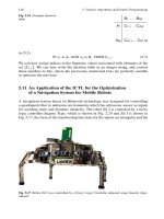
shafting system [80–82]. In this chapter, the marine shafting system is modeled as a
chained multiple mass-spring-damper system [82].
In recent years, research on control of marine vessels has been extended to include
the thruster dynamics in the control design. The main focus of marine propulsion con-
trol is on achieving the desired position and velocity for the marine vessel through the
control of shaft speed for fixed pitch (FP) propellers and pitch for controllable pitch
(CP) propellers. Nonlinear output feedback control of propeller shaft speed was de-
veloped in [83] for underwater vehicles where variations in the propeller thrusts due to
unsteady flow effects were compensated for through the estimation of the propeller ax-
ial flow velocity. Recent developments in marine propulsion control have shifted from
the control of shaft speed or propeller pitch to the control of power from the drive sys-
6
1.2. Adaptive NN Control of Marine Shafting System
tem in order to achieve the desired thrust [84] through a mapping from propeller force to
torque/power. This method has been shown to achieve improved performance in moder-
ate seas over conventional shaft speed controls. Although the marine propulsion control
has been an active area of research, the design of an effective control strategy to actively
minimize torsional vibrations within the shafting systems have received relatively little
attention.
Hydrodynamic forces acting on the propeller are highly nonlinear and subjected to
variations due to the diverse operating conditions such as air suction, cavitation and
partial/full emergence of the propellers [83–85]. Furthermore, torsional stiffness of the
drive shaft will be subjected to changes during operation due to the mechanical wear
and tear of the shafting system. Traditional adaptive controls are generally useful when

dealing with systems whose dynamics can be expressed in the linear-in-parameters
form, for which the regressor is exactly known and the uncertainty is parametric and
time-invariant. Such a restriction is clearly ill-suited for this system. To overcome
this limitation, approximation-based control techniques is adopted to compensate for
functional uncertainties in the dynamic model of the shafting system.
In this case study, an adaptive NN control using decoupled backstepping is first
presented followed by an adaptive NN control using DSC to address the issues associ-
ated with the control of marine shafting systems highlighted above. The control objec-
tive for both approaches is to track a desired propeller trajectory while simultaneously
minimizing torsional vibrations within the shafting system, in the presence of paramet-
ric/functional uncertainties and disturbances. NNs are utilized to compensate for the
parametric uncertainties in the system model, the unknown hydrodynamic forces acting
on the propeller as well as the frictional forces present in the shafting system. In the
implementation of the adaptive NN control using decoupled backstepping, it is noted
that the complexities involved in the control design increases with each subsequent step
of the backstepping due to the required computation of the partial derivatives for the
NNs. Moreover, when applying RBF NNs in the backstepping process, this problem
translates into more NN inputs required which leads to an exponential increase in the
size of the NNs for each additional element considered in the model. When modelling
7
1.3. Thesis Outline
the shafting system as a multiple mass-spring-damper system, a large number of ele-
ments in the model may be required to achieve an accurate representation of the phys-
ical system, thus compounding the problems associated with traditional and decoupled
backstepping. Comparatively, when applying DSC, the “explosion of terms” problem
experienced in backstepping control can be avoided. In addition, when applying back-
stepping in the presence of functional uncertainties in the system model leads to the
uncertainties appearing in the time derivatives of the virtual controls. In the decou-
pled backstepping approach, due to the structure of the dynamic model considered and
the approach adopted, the NNs in every alternate step of the backstepping are required

exclusively for the approximation of the time derivatives of the virtual controls. In con-
trast, the time derivatives of the virtual controls are approximated by first-order filters
in dynamic surface control, thus removing the need of NNs for every alternate step in
the backstepping which effectively reduces the number of NNs required in the system
by half. Therefore, through the application of dynamic surface control technique, it is
possible to reduce the number of NNs required as well as reducing the size of the NNs
in the control.
1.3 Thesis Outline
The remainder of this thesis is organized as follows:
In Chapter 2, an AVSC using decoupled backstepping approach is presented for a
class of uncertain, non-affine and nonlinear systems with the control objective to track
a desired trajectory. In this chapter, the system model and some mathematical prelimi-
naries are presented, followed by the control design. Subsequently, a stability analysis
of the closed-loop system is presented where all the closed-loop signals are shown to
be bounded. Finally, a simulation study is presented to illustrate the effectiveness of the
proposed control.
In Chapter 3, an extension of the work in Chapter 2 is presented. An AVSC is
developed for the same class of uncertain, non-affine and nonlinear systems using a
modified coupled backstepping approach where the coupling terms are handled in the
8
1.3. Thesis Outline
next step of the backstepping without resulting in circular design. In this approach, an
assumption that was required in the design of the decoupled backstepping approach can
be relaxed. Simulation results shows the effectiveness of the proposed approach and
the differences, in terms of the performance and implementation issues, between the
decoupled and coupled approaches are highlighted.
In Chapter 4, an extension of the work in Chapters 2 and 3 is presented. An AVSC
is developed for the same class of uncertain, non-affine and nonlinear systems using a
dynamic surface approach where the derivatives of the virtual controls are approximated
with first order filters. In this approach, the derivatives of the virtual controls need not

be approximated by the NNs, thus reducing the number of inputs to the NNs which
in turn reduces the size of the NNs. Simulation results are presented to illustrate the
effectiveness of the proposed approach.
In Chapter 5, an application study is conducted where the system considered is
a marine shafting system. The model of the marine shafting system is first presented
where the system model contains parametric/functional uncertainties and disturbances.
The control objective is to achieve trajectory tracking while simultaneously minimiz-
ing torsional vibrations within the shafting system. In an extension on the study of
decoupled backstepping and DSC is presented in previous chapters, two adaptive NN
controls are developed where the first control is designed using decoupled backstep-
ping. Subsequently, an adaptive NN control using DSC is presented with the same
control objective. Finally, a simulation study for for both approaches is conducted and
a comparative study on the two approaches is presented where the performance and
implementation issues are highlighted.
Finally, a summary of the work presented in this thesis is given in Chapter 6 to-
gether with a review of the contributions made in this thesis and a recommendation for
future work.
9
Chapter 2
AVSC with Decoupled Backstepping
2.1 Introduction
In this chapter, adaptive variable structure control (AVSC) is investigated for a class
of nonlinear pure-feedback single-input single-output (SISO) systems with unknown
nonlinear functions based on neural network parametrization. The non-affine nonlinear
control problem is challenging due to the relatively fewer mathematical tools available
in comparison with that for affine nonlinear systems. In particular, it is difficult to
construct control laws because pure-feedback systems have no affine appearance of the
variables which can be used as virtual controls.
This chapter is organized as follows: In Section 2.2 the system considered is pre-
sented followed by some definitions, Lemmas and assumptions that are required in the

subsequent design and stability analysis. Thereafter, the structure and definition of the
NN that will be used in the control design is presented. Subsequently, in Section 2.4, the
design procedures for the proposed AVCS utilizing decoupled backstepping is presented
and followed by the stability analysis which is presented in Section 2.5. A simulation
study is presented in Section 2.6 to demonstrate the effectiveness of the control.
10
2.2. Problem Formulation and Preliminaries
2.2 Problem Formulation and Preliminaries
Consider the following class of uncertain nonlinear non-affine pure-feedback single-
input single-output (SISO) systems:
˙x
i
= f
i
(¯x
i
, x
i+1
) for i = 1, , n − 1
˙x
n
= f
n
(¯x
n
, u)
y = x
1
(2.1)
where f

i
(·) is an unknown smooth function; and ¯x
i
= [x
1
, , x
i
]
T
∈ R
i
, y ∈ R and
u ∈ R, (i = 1, , n) are the state variables, system output and input, respectively.
The control objective is to design an adaptive controller for system (2.1) such that
the output y follows a desired trajectory y
d
, while all the signals in the closed-loop
systems are bounded.
Assumption 2.2.1. The desired trajectory y
d
is known, bounded and C
n
continuously
differentiable.
Definition 2.2.1. [86] The solution of (2.1) is Semi-Globally Uniformly Ultimately
Bounded (SGUUB) if, for any compact set Ω
0
, there exists an S > 0 and T = T (S, X(t
0
))

such that X(t) ≤ S for all X(t
0
) ∈ Ω
0
and t ≥ t
0
+ T .
Lemma 2.2.1. Mean Value Theorem [87]: Assume that f(x, y) : R
n
× R → R has a
derivative at each point of an open set R
n
×(a, b), and assume also that it is continuous
at both endpoints y = a and y = b. Then, there is a point ξ ∈ (a, b) such that
f(x, b) − f(x, a) = f

(x, ξ)(b − a).
From Lemma 2.2.1, the non-affine functions in (2.1) can be written as
f
i
(¯x
i
, x
i+1
) − f
i
(¯x
i
, x
0

i+1
) =
∂f
i
(¯x
i
, x
i+1
)
∂x
i+1



x
i+1
=x
θ
i
i+1
x
i+1
f
n
(¯x
n
, u) − f
n
(¯x
n

, u
0
) =
∂f
n
(¯x
n
, u)
∂u
|
u=u
θ
n
u (2.2)
where x
0
i
for i = 2, ··· , n and u
0
are design constants. For a more effective control
11
2.2. Problem Formulation and Preliminaries
design, the values for x
0
i
and u
0
should be chosen such that x
0
i

and u
0
lies within their
corresponding operating region, for example, the value x
0
i
should lie within the oper-
ating region of the state x
i
. For convenience, the control u is denoted as x
n+1
, and
x
θ
i
i+1
= θ
i
x
i+1
+ (1 − θ
i
)x
0
i+1
is some unknown point between x
i+1
and x
0
i+1

in which
θ
i
is a time-varying parameter satisfying 0 < θ
i
(t) < 1 (i = 1, 2, , n) ∀ t ≥ 0.
Substituting (2.2) into (2.1), the system dynamics can be rewritten as
˙x
i
= f
i
(¯x
i
, x
0
i+1
) + g
i
(¯x
i
, x
θ
i
i+1
)x
i+1
for i = 1, , n − 1
˙x
n
= f

n
(¯x
n
, u
0
) + g
n
(¯x
n
, u
θ
n
)u
y = x
1
(2.3)
where
g
i
(¯x
i
, x
θ
i
i+1
) =
∂f
i
(¯x
i

, x
i+1
)
∂x
i+1



x
i+1
=x
θ
i
i+1
(i = 1, , n − 1)
g
n
(¯x
n
, u
θ
n
) =
∂f
n
(¯x
n
, u)
∂u
|

u=u
θ
n
Remark 2.2.1. By applying Mean Value Theorem, the system dynamics (2.1) can be
rewritten in the form of (2.3), which can be viewed as another pure-feedback system
since the input gain functions of (2.3) are still partially non-affine due to the presence
of x
θ
i
i+1
in g
i
.
Remark 2.2.2. The key distinction between the Mean Value Theorem and the Taylor
series expansion is that the former is valid globally, while the latter is only valid locally
around a specified point. In particular, with Taylor series expansion, a smooth function
would be approximated at one point with a high-order approximating error. On the
other hand, with Mean Value Theorem, this function would be expanded between two
points without a high-order approximating error. Unlike the Taylor series expansion,
which usually yields local stability, the Mean Value Theorem, as used in our approach,
yields semi-global stability, as will be shown in our main results in Theorem 2.5.1.
Remark 2.2.3. If coupled backstepping design [27] was applied for the control of equa-
12
2.2. Problem Formulation and Preliminaries
tion (2.3), it would result in a circular control design since the control gain functions
are still non-affine in control. In the following, decoupled backstepping design [88, 89]
will be employed for this problem.
Lemma 2.2.2. [90] For bounded initial conditions, if there exists a C
1
continuous and

positive definite Lyapunov function V (x, t) satisfying V (x) ≤ V (x, t) ≤
¯
V (x),
such that
˙
V (x, t) ≤ −ρ
1
V (x, t) + ρ
2
, where V ,
¯
V : R
n
→ R are class K functions and
ρ
1
, ρ
2
are positive constants, then the solution x = 0 is uniformly bounded.
Assumption 2.2.2. The signs of g
i
(·) ∈ R in (2.3) are known, and there exist constants
g
min
> 0 and g
max
> 0 such that ∀ ¯x
n
∈ Ω
x

⊂ R
n
, we have g
max
≥ |g
i
(·)| (i =
1, 2, , n − 1) and ∀ ¯x
n
∈ R
n
, u ∈ R, |g
i
(·)| ≥ g
min
(i = 1, 2, , n) where Ω
x
is
a compact set. Without loss of generality, we assume that g
i
(·) > 0, ∀ ¯x
n
∈ R
n
and
u ∈ R.
Remark 2.2.4. The smooth function g
i
(·) is strictly either positive or negative accord-
ing to Assumption 2.2.2. Since x

θ
i
i+1
is not available, g
i
(¯x
i
, x
θ
i
i+1
) cannot be approxi-
mated by NNs. However, the bounds of g
i
(¯x
i
, x
θ
i
i+1
) will be used in the control system
design rather than g
i
(¯x
i
, x
θ
i
i+1
). It should be emphasized that g

i
(¯x
i
, x
θ
i
i+1
) is only re-
quired for analytical purposes, and will not be approximated by neural networks at
all.
The following technical lemmas are required in the subsequent control design and
stability analysis.
Lemma 2.2.3. For a, b ∈ R
+
, the following inequality holds
ab
a + b
≤ a (2.4)
Lemma 2.2.4. Consider a first-order dynamical system
˙s = −λs + φ(t) (2.5)
13
2.2. Problem Formulation and Preliminaries
where φ(t) is a bounded and continuous nonnegative function and λ is a positive con-
stant. If a nonnegative initial value s(0) is chosen, then the solution s(t) is nonnegative
for all t > 0.
Lemma 2.2.5. For uniformly continuous z(t) ∈ R, t ∈ [0, +∞), if





z(t) + k

t
0
z(τ )dτ




≤ c (2.6)
then z(t) and

t
0
z(τ )dτ are both bounded in t ∈ [0, +∞) and satisfy the following
relationships





t
0
z(τ )dτ




≤
c

k
(1 − e
−kt
) ≤
c
k
|z(t)| ≤ c(2 − e
−kt
) ≤ 2c (2.7)
where k and c are positive constants.
Proof. Defining ω(t) =

t
0
z(τ )dτ, ˙ω = z(t) and ω(0) = 0 lead to
−c ≤ ˙ω + kω ≤ c (2.8)
Solving the inequalities result in
ω(0)e
−kt
−
c
k
(1 − e
−kt
) ≤ ω ≤ ω(0)e
−kt
+
c
k
(1 − e

−kt
) (2.9)
That is
−
c
k
≤ −
c
k
(1 − e
−kt
) ≤

t
0
z(τ )dτ ≤
c
k
(1 − e
−kt
) ≤
c
k
(2.10)
With (2.8) and (2.10), we have
−2c ≤ −c(2 − e
−kt
) ≤ z ≤ c(2 −e
−kt
) ≤ 2c (2.11)

This completes the proof.
14
2.3. Neural Networks and Parametrization
2.3 Neural Networks and Parametrization
Functional approximators can be represented as multi-layer feedforward networks which
may be linearly- or nonlinearly-parameterized. A class of linearly parameterized feed-
forward approximators used to approximate the continuous function f(Z) : R
q
→ R
may be represented as follows:
f
nn
(Z) = W
T
S(Z) (2.12)
where the vector Z = [z
1
, ··· , z
q
]
T
∈ R
q
are the input variables to the approximator,
W ∈ R
l
is a vector of adaptable weights and S(Z) = [s
1
(Z), ··· , s
l

(Z)]
T
∈ R
l
is a
vector of known continuous (linear or nonlinear) basis functions. In this thesis, Radial
Basis Functions (RBF) NNs are used where the basis functions s
i
(Z) are chosen as the
commonly used Gaussian functions,
s
i
(Z) = exp

−(Z − µ
i
)
T
(Z − µ
i
)
λ
2
i

, i = 1, ··· , l (2.13)
where µ
i
= [µ
i1

, µ
i2
, ··· , µ
iq
]
T
is the center of the receptive field for node i and λ
i
is
the width of the Gaussian function.
Universal approximation results in [39] indicate that if l is chosen sufficiently large,
W
T
S(Z) can approximate any continuous function, f(Z), to any desired accuracy over
a compact set Ω
Z
⊂ R
q
to any arbitrary degree of accuracy.
f(Z) = W
∗
T
S(Z) + ε(Z), ∀Z ∈ Ω
Z
⊂ R
q
(2.14)
where W
∗
is the ideal constant weight vector and ε(Z) is the approximation error for the

special case where W = W
∗
which is bounded over the compact set, i.e., |ε(Z)| ≤ ¯ε,
∀Z ∈ Ω
Z
where ¯ε > 0 is an unknown constant. The ideal weight vector W
∗
, an artificial
quantity required for analytical purposes, is defined as the value of W that minimizes
15
2.3. Neural Networks and Parametrization
|ε(Z)| for all Z ∈ Ω
Z
⊂ R
q
, i.e.,
W
∗
:= arg min
W ∈R
l
[ sup
Z∈Ω
Z
|f(Z) −W
T
S(Z)|] (2.15)
Remark 2.3.1. Based on the definition of the ideal weight vectors W
∗
(2.15), NN ap-

proximation error ε (2.14) and ∀ Z ∈ Ω, there exists unknown constants w
max
where
w
max
satisfies
w
max
≥ |w
∗
i
|, i = 1, , l (2.16)
and w
∗
i
is the ith NN weight in the ideal weight vector W
∗
.
Based on the technique used in Section 4.3.1 of [56], an upper bound for the neural
network parametrization can be obtained, from which there is only one positive param-
eter to be adapted. From (2.14),
W
∗T
S(Z) + ε(Z) ≤


W
∗T
S(Z)



+ |ε(Z)|
≤
l

m=1
|s
m
(Z)|w
max
+ ¯ε
≤ ψ
∗
β(Z) (2.17)
where
β(Z) =
l

m=1

s
2
m
(Z) +  + 1
ψ
∗
= max{¯ε, w
max
} (2.18)
and  is a positive design constant.

Remark 2.3.2. The 2-norm is used to obtain β(Z) so that it is differentiable, which is
important in the subsequent control design based on backstepping.
16