Evolutionary multi objective optimization in investment portfolio management
Bạn đang xem bản rút gọn của tài liệu. Xem và tải ngay bản đầy đủ của tài liệu tại đây (4.2 MB, 228 trang )
EVOLUTIONARY MULTI-OBJECTIVE OPTIMIZATION
IN INVESTMENT PORTFOLIO MANAGEMENT
CHIAM SWEE CHIANG
(B.Eng (Hons.), NUS)
A THESIS SUBMITTED
FOR THE DEGREE OF DOCTOR OF PHILOSOPHY
DEPARTMENT OF ELECTRICAL & COMPUTER ENGINEERING
NATIONAL UNIVERSITY OF SINGAPORE
2009
Abstract
Many real-world problems involve the simultaneous optimization of several competing objectives
and constraints that are difficult, if not impossible, to solve without the aid of powerful optimization
algorithms. As no one solution is optimal to all objective in the presence of conflicting specifications,
the optimization algorithms must b e capable of generating a set of alternative solutions, representing
the tradeoffs between the objectives. Evolutionary algorithms, a class of population-based stochastic
search technique, have shown general success in solving complex real-world multi-objective optimiza-
tion problems, where conventional optimization tools failed to work well. Its main advantage lies
in its capability to sample multiple candidate solutions simultaneously, hence enabling the entire
set of Pareto-optimal solutions to be approximated in a single algorithmic run. Much work has
been devoted to the development of multi-objective evolutionary algorithms in the past decade and
it is increasingly finding application to the diverse fields of engineering, bioinformatics, logistics,
economics, finance, and etc.
This thesis focuses particularly on investment portfolio management, an important subject in
the field of economics and finance, where the central theme is the professional management of an
appropriate mix of financial assets to satisfy specific investment goals. The decision process will
typically involve issues such as asset allocation, security selection, performance measurement, man-
agement styles and etc. Due to the complexity of these issues, classical optimization tools from
the realm of operations research are restricted to a limited set of problems and/or the optimization
models have to accept strong simplifications. These restrictions have thus motivated the develop-
ment and application of evolutionary optimization techniques for this purpose. As such, the primary
motivation of this thesis is to provide a comprehensive treatment on the design and application of
multi-objective evolutionary algorithms to address the several key issues involved with investment
portfolio management, namely asset allocation and portfolio management style.
For asset allo cation, the mean-variance model developed by Harry Markowitz, widely regarded
as the foundation of modern portfolio theory, is considered to provide the quantitative framework for
this optimization problem. A generic multi-objective evolutionary algorithm designed specifically for
portfolio optimization is proposed and its feasibility is evaluated based on a rudimentary instantiation
of the mean-variance model. Avenues to incorporate user preferences into the portfolio construction
process are examined also. In addition, real-world constraints arising from business/industry regu-
lations and practical concerns are incorporated to enhance the realism of the mean-variance model
and the impacts on the efficient frontier are studied.
The second part of this work is concerned with portfolio management style, which can be broadly
classified as active and passive. While active management relies on the belief that excess yields over
i
Abstract ii
market average are attainable by exploiting market inefficiencies, passive management centers on ef-
ficient financial markets and aims to replicate returns-risk profiles similar to market indices. For the
former, security selection through technical analysis is studied, where a multi-objective evolutionary
platform is developed to optimize technical trading strategies capable of yielding high returns at
minimal risk. Popular technical indicators used commonly in real-world practices are used as the
building blocks for these strategies, which hence allow the examination of their trading characteris-
tics and behaviors on the evolutionary platform. In the aspect of passive management, a realistic
instantiation of the index tracking optimization problem that accounted for stochastic capital injec-
tions, practical transactions cost structures and other real-world constraints is formulated and used
to evaluate the feasibility of the proposed multi-objective evolutionary platform that simultaneously
optimized tracking performance and transaction costs throughout the investment horizon.
Acknowledgements
First and foremost, I will like to thank my thesis supervisor, Professor Tan Kay Chen for introducing
me to the wonderful field of computational intelligence and his continuous support and guidance
throughout my course of study. His understanding, encouragments and personal guidances provided
the basis for this thesis. I will also like to thank my co-supervisor, Professor Abdullah Al Mamun
for his important support throughout this work.
All my lab buddies at the Control and Simulation laboratory made it a convivial place to work.
In particular (in order of seniority), I will like to TAC-Q Chi Keong for showing me the way of
research, Dasheng for his invaluable contributions to the research group, Eujin who accompanied
me to the world of finance, Brian AND Chun Yew for the soap and drama, Hanyang for keeping me
on course and Chin Hiong for his tips! Jokes aside, this bunch of great folks, as well all others in
C&S lab, have inspired me in research and life through our interactions and stimulating discussions
during the long hours in the lab. Thanks!
I owe my loving thanks to my wife Pricilla, who has been extremely kind and understanding
during this period of my life. Without her encouragement and understanding, it would have been
impossible for me to finish this work. Also, my special gratitude is due to my entire family, notably
my two sisters Valerie and Siew Sze for providing me a loving environment.
Lastly and most importantly, I wish to thank my parents, Tony and Judy. They bore me, raised
me, supported me, taught me, and loved me. To them, I dedicate this thesis.
iii
Publications
1. S. C. Chiam, K. C. Tan and A. A. Mamun, “A Memetic Model of Evolutionary PSO for
Computational Finance Applications,” Expert Systems With Applications, vol. 36, no. 2, pp.
3695-3711, 2009.
2. S. C. Chiam, K. C. Tan and A. A. Mamun, “Investigating technical trading strategy via an
multi-objective evolutionary platform,” Expert Systems with Applications, vol. 36, no. 7, pp.
10408-10423, 2009.
3. K. C. Tan, S. C. Chiam, A. A. Mamun and C. K. Goh, “Balancing Exploration and Exploitation
with Adaptive Variation for Evolutionary Multi-objective Optimization,” European Journal
of Operational Research, vol. 197, no. 2, pp. 701-713, 2009.
4. S. C. Chiam, K. C. Tan, C. K. Goh and A. A. Mamun, “Improving Locality in Binary Rep-
resentation via Redundancy,” IEEE Transactions on Systems, Man and Cybernetics, Part B
(Cybernetics), vol. 38, no. 3, pp. 808-825, 2008.
5. S. C. Chiam, K. C. Tan and A. A. Mamun, “Evolutionary multi-objective portfolio optimization
in practical context,” International Journal of Automation and Computing, vol. 5, no. 1, pp.
67-80, 2008.
6. S. C. Chiam, K. C. Tan and A. A. Mamun, “Molecular Dynamics Optimizer,” Fourth Interna-
tional Conference on Evolutionary Multi-Criterion Optimization, Matsushima, Japan, March
5-8, pp. 302-316, 2007.
7. S. C. Chiam, K. C. Tan and A. A. Mamun, “Multiobjective Evolutionary Neural Networks for
Time Series Forecasting,” Fourth International Conference on Evolutionary Multi-Criterion
Optimization, Matsushima, Japan, March 5-8, pp. 346-360, 2007.
8. S. C. Chiam, C. K. Goh and K. C. Tan, “Adequacy of Empirical Performance Assessment
for Multiobjective Evolutionary Optimizer,” Fourth International Conference on Evolutionary
Multi-Criterion Optimization, Matsushima, Japan, March 5-8, pp. 893-907, 2007.
9. C. Y. Cheong, S. C. Chiam and C. K. Goh, “Eliminating Positional Dependency in Binary
Representation via Redundancy,” 2007 IEEE Symposium on Foundations of Computational
Intelligence Article, Honolulu 1-5 April, pp. 251-258, 2007.
iv
Publications v
10. S. C. Chiam, K. C. Tan, A. A. Mamun and Y. L. Low, “A Realistic Approach to Evolutionary
Multi-objective Portfolio Optimization,” IEEE Congress on Evolutionary Computation 2007,
Singapore, September 25-28, pp. 204-211, 2007.
11. S. C. Chiam, C. K. Goh and K. C. Tan, “Issues of Binary Representation in Evolutionary
Algorithms, ” The 2nd IEEE International Conference on Cybernetics & Intelligent Systems,
Bangkok, Thailand, June 7-9, 2006.
12. C. K. Goh, S. C. Chiam and K. C. Tan, “An Investigation on Noisy Environments in Evolution-
ary Multi-Objective Optimization, ” The 2nd IEEE International Conference on Cybernetics
& Intelligent Systems, Bangkok, Thailand, June 7-9, 2006.
13. E. J. Teoh, S. C. Chiam, C. K. Goh and K. C. Tan, “Adapting evolutionary dynamics of
variation for multi-ob jective optimization,” IEEE Congress on Evolutionary Computation
2005, Edinburgh, UK, vol. 2, pp. 1290-1297,2005.
14. C. K. Goh, K. C. Tan, D. S. Liu, S. C. Chiam, “A competitive and cooperative co-evolutionary
approach to multi-objective particle swarm optimization algorithm design,” European Journal
of Operational Research, accepted.
Contents
Abstract i
Acknowledgements iii
Publications iv
Contents vi
List of Figures x
List of Tables xvi
1 Investment Portfolio Management 1
1.1 Asset Allocation via Mean-Variance Analysis . . . . . . . . . . . . . . . . . . . . . . 2
1.1.1 Mean-VarianceModel 2
1.1.2 Limitations of Markowitz Model . . . . . . . . . . . . . . . . . . . . . . . . . 5
1.2 Investment Portfolio Management Styles . . . . . . . . . . . . . . . . . . . . . . . . . 7
1.2.1 Active Portfolio Management . . . . . . . . . . . . . . . . . . . . . . . . . . . 7
1.2.2 Passive Portfolio Management . . . . . . . . . . . . . . . . . . . . . . . . . . 8
1.3 ThesisOverview 9
1.4 Summary 11
2 Evolutionary Multi-Objective Optimization 12
2.1 Introduction 12
2.2 Multi-Objective Optimization . . . . . . . . . . . . . . . . . . . . . . . . . . . . . . . 13
2.2.1 ProblemDefinition 13
2.2.2 ParetoOptimality 14
2.2.3 Optimization Goals . . . . . . . . . . . . . . . . . . . . . . . . . . . . . . . . 16
2.3 Evolutionary Optimization . . . . . . . . . . . . . . . . . . . . . . . . . . . . . . . . 18
2.3.1 Evolutionary Algorithm . . . . . . . . . . . . . . . . . . . . . . . . . . . . . . 18
2.3.2 Particle Swarm Optimization . . . . . . . . . . . . . . . . . . . . . . . . . . . 20
2.3.3 Multi-Objective Evolutionary Algorithm . . . . . . . . . . . . . . . . . . . . . 22
2.3.4 Memetic Algorithm . . . . . . . . . . . . . . . . . . . . . . . . . . . . . . . . 23
2.4 Summary 26
vi
CONTENTS vii
3 Extending MOEA for Portfolio Optimization 27
3.1 Introduction 27
3.2 Chromosomal Representation for Portfolio Structure . . . . . . . . . . . . . . . . . . 27
3.2.1 Order-Based Representation . . . . . . . . . . . . . . . . . . . . . . . . . . . . 28
3.2.2 Empirical Study & Analysis . . . . . . . . . . . . . . . . . . . . . . . . . . . . 29
3.3 VariationOperation 34
3.3.1 Crossover and Mutation Operators . . . . . . . . . . . . . . . . . . . . . . . . 34
3.3.2 Empirical Study & Analysis . . . . . . . . . . . . . . . . . . . . . . . . . . . . 36
3.4 LocalSearchOperator 41
3.4.1 EA-PSO Memetic Models . . . . . . . . . . . . . . . . . . . . . . . . . . . . . 43
3.4.2 Knapsack Problem as a Proxy for Portfolio Optimization . . . . . . . . . . . 45
3.4.3 SimulationSetup 47
3.4.4 Simulation Result & Discussion . . . . . . . . . . . . . . . . . . . . . . . . . . 49
3.4.5 Effects of Varying Problem Settings . . . . . . . . . . . . . . . . . . . . . . . 52
3.5 Dynamic Archiving Operator . . . . . . . . . . . . . . . . . . . . . . . . . . . . . . . 56
3.5.1 Dynamic Optimization . . . . . . . . . . . . . . . . . . . . . . . . . . . . . . . 56
3.5.2 Handling Dynamism in Evolutionary Optimization . . . . . . . . . . . . . . . 57
3.5.3 SimulationSetup 60
3.5.4 Simulation Result & Discussion . . . . . . . . . . . . . . . . . . . . . . . . . . 61
3.6 Summary 70
4 Mean-Variance Analysis and Preference Handling 72
4.1 Introduction 72
4.2 Markowitz Mean-Variance Model . . . . . . . . . . . . . . . . . . . . . . . . . . . . 72
4.3 Optimization Techniques for Portfolio Optimization . . . . . . . . . . . . . . . . . . 75
4.4 Evolutionary Multi-Objective Portfolio Optimization . . . . . . . . . . . . . . . . . . 77
4.4.1 SimulationSetup 77
4.4.2 Performance Metrics . . . . . . . . . . . . . . . . . . . . . . . . . . . . . . . . 78
4.4.3 Simulation Result & Discussion . . . . . . . . . . . . . . . . . . . . . . . . . 79
4.5 Handling Preferences in Portfolio Optimization . . . . . . . . . . . . . . . . . . . . . 85
4.5.1 Preferences in Multi-Objective Optimization . . . . . . . . . . . . . . . . . . 85
4.5.2 Capital Asset Pricing Model . . . . . . . . . . . . . . . . . . . . . . . . . . . 86
4.5.3 SimulationSetup 88
4.5.4 Simulation Result & Discussion . . . . . . . . . . . . . . . . . . . . . . . . . . 89
4.6 Summary 94
CONTENTS viii
5 Handling Realistic Constraints in Portfolio Optimization 96
5.1 Introduction 96
5.2 Review of Realistic Constraints in Portfolio Optimization . . . . . . . . . . . . . . . 97
5.2.1 Floor and Ceiling Constraints . . . . . . . . . . . . . . . . . . . . . . . . . . . 98
5.2.2 Cardinality Constraint . . . . . . . . . . . . . . . . . . . . . . . . . . . . . . . 98
5.2.3 Round-lot Constraint . . . . . . . . . . . . . . . . . . . . . . . . . . . . . . . 99
5.2.4 TurnoverConstraint 99
5.2.5 TradingConstraint 99
5.2.6 TransactionCosts 100
5.3 Handling Cardinality Constraint with Buy-in Threshold . . . . . . . . . . . . . . . . 101
5.3.1 Constraint Handling Technique for Buy-In Threshold . . . . . . . . . . . . . 101
5.3.2 Constraint Handling Technique for Cardinality Constraint . . . . . . . . . . . 102
5.3.3 Simulation Result & Discussion . . . . . . . . . . . . . . . . . . . . . . . . . . 103
5.4 Handling Round-Lot Constraint with Transaction Costs . . . . . . . . . . . . . . . . 108
5.4.1 Problem Formulation . . . . . . . . . . . . . . . . . . . . . . . . . . . . . . . 110
5.4.2 Simulation Result & Discussion . . . . . . . . . . . . . . . . . . . . . . . . . . 112
5.5 Summary 117
6 Investigating Technical Trading Strategies via EMOO 118
6.1 Introduction 118
6.2 Technical Trading Strategies . . . . . . . . . . . . . . . . . . . . . . . . . . . . . . . . 120
6.3 Multi-Objective Evolutionary Platform for ETTS . . . . . . . . . . . . . . . . . . . . 124
6.3.1 Variable-length Representation for Trading Agents . . . . . . . . . . . . . . . 125
6.3.2 Objective Functions . . . . . . . . . . . . . . . . . . . . . . . . . . . . . . . . 126
6.3.3 Fitness Evaluation . . . . . . . . . . . . . . . . . . . . . . . . . . . . . . . . . 129
6.3.4 Pareto Fitness Ranking . . . . . . . . . . . . . . . . . . . . . . . . . . . . . . 133
6.3.5 Variation Operation . . . . . . . . . . . . . . . . . . . . . . . . . . . . . . . . 134
6.3.6 AlgorithmicFlow 136
6.4 Simulation Result & Discussion . . . . . . . . . . . . . . . . . . . . . . . . . . . . . 137
6.4.1 Performance Comparison between Individual TI and Hybrid TI . . . . . . . . 138
6.4.2 Correlation Analysis between Training and Test Performance . . . . . . . . . 148
6.4.3 Generalization Performance . . . . . . . . . . . . . . . . . . . . . . . . . . . . 151
6.5 Summary 154
CONTENTS ix
7 Dynamic Index Tracking via Multi-Objective Evolutionary Optimization 156
7.1 Introduction 156
7.2 IndexTracking 158
7.2.1 Variable Notations . . . . . . . . . . . . . . . . . . . . . . . . . . . . . . . . . 158
7.2.2 Problem Definition . . . . . . . . . . . . . . . . . . . . . . . . . . . . . . . . . 161
7.2.3 Objective Functions . . . . . . . . . . . . . . . . . . . . . . . . . . . . . . . . 163
7.2.4 Constraints 165
7.3 Multi-Objective Evolutionary Optimization . . . . . . . . . . . . . . . . . . . . . . . 165
7.3.1 Chromosomal Representation . . . . . . . . . . . . . . . . . . . . . . . . . . . 166
7.3.2 SelectionProcess 167
7.3.3 Dynamic Archiving Operator . . . . . . . . . . . . . . . . . . . . . . . . . . . 169
7.3.4 Algorithmic Flow of Index Tracking System . . . . . . . . . . . . . . . . . . . 170
7.4 Single-Period Index Tracking . . . . . . . . . . . . . . . . . . . . . . . . . . . . . . . 172
7.4.1 Data Sets & Simulation Setting . . . . . . . . . . . . . . . . . . . . . . . . . . 172
7.4.2 Simulation Result & Discussion . . . . . . . . . . . . . . . . . . . . . . . . . . 173
7.5 Multi-Period Index Tracking . . . . . . . . . . . . . . . . . . . . . . . . . . . . . . . . 176
7.5.1 Data Sets & Simulation Setting . . . . . . . . . . . . . . . . . . . . . . . . . . 177
7.5.2 Simulation Result & Discussion . . . . . . . . . . . . . . . . . . . . . . . . . . 178
7.6 Summary 187
8 Conclusions 189
8.1 Contributions 189
8.2 FutureWorks 191
List of Figures
1.1 Daily price series of DBS and UOB (i.e. the two largest bank stocks in terms of
capitalization value in the Straits Times Index, Singapore) for the period between
01012008and05082008. 3
1.2 Plot showing the risk-return profiles by considering different weights combinations in
the two-asset (i.e. DBS and UOB) portfolio optimization problem. Efficient frontier
ishighlightedinbold. 5
2.1 Evaluation mapping function between the decision variable space and objective space
inMOO 14
2.2 Illustration of the Pareto Dominance relationship between candidate solutions and the
referencesolution. 16
2.3 Illustration of the various concepts of Pareto Optimality. . . . . . . . . . . . . . . . . 17
2.4 Plots comparing two different sets of solutions (white circles versus black circles),
where each plot illustrates the superiority of the set of white circles over the black
circles in terms of (a) proximity, (b) Spread and (c) Spacing. . . . . . . . . . . . . . 18
2.5 Algorithmic flow of a general MOEA presented as a flowchart. . . . . . . . . . . . . . 20
3.1 A chromosomal instance for the ordered based representation proposed based on eight
assetsavailable 28
3.2 Fitness evaluation for the chromosome in Figure 3.1. Assets are iteratively added into
the portfolio until the accumulated weights exceed one. The various weights in the
portfolio are then normalized to one to satisfy the budget constraint. . . . . . . . . . 29
3.3 Average portfolio size (maximum 30) for 100,000 randomly generated chromosomes
with different weight limits. ‘0 – 0.2’denotes the case where each chromosome is
assigned a different Wmax value, derived from a uniform distribution on the interval
[0,0.2]. 31
3.4 Distribution of portfolio size (maximum 30) for 100,000 randomly generated chromo-
somes with different representation schemes. . . . . . . . . . . . . . . . . . . . . . . . 32
3.5 Box plots illustrating the p ortfolio size distribution (maximum 30) for 100,000 ran-
domly generated chromosomes with different value of K
T arget
. 33
3.6 Distribution of portfolio size (maximum 30) for 100,000 randomly generated chromo-
somes with different targeted range. . . . . . . . . . . . . . . . . . . . . . . . . . . . 34
x
LIST OF FIGURES xi
3.7 Single-point crossover. Genes after the crossover point are swapped between the two
parentchromosomes 35
3.8 Bit-swap mutation i.e. position of randomly chosen genes are swapped. . . . . . . . . 35
3.9 Empirical Distribution of (a) MI and (b) MI > 0 for 100,000 randomly generated
chromosomes under different mutation operations. . . . . . . . . . . . . . . . . . . . 38
3.10 Empirical distributions of (a) E(MI
k
|MI
k
> 0) and (b)σ(MI
k
|MI
k
> 0) over the number
of mutation, k, for the various mutation operators . . . . . . . . . . . . . . . . . . . 39
3.11 Empirical Distribution of CI (left) and CI> 0 (right) for 100,000 randomly generated
chromosomes with different XO scheme . . . . . . . . . . . . . . . . . . . . . . . . . 41
3.12 Fitness attained by the various algorithms after 500,000 fitness evaluation illustrated
inboxplots 50
3.13 Evolutionary traces of the fitness and hamming distance for the best solution of (a)EA,
(b) EAPSO20a and (c) EAPSO100a in one of the simulation run. . . . . . . . . . . . 51
3.14 Mean fitness improvements whenever PSO was triggered at different fitness evaluations
by EALS-20a, EALS-50a, EALS-100a and EALS-500a. . . . . . . . . . . . . . . . . . 52
3.15 Mean fitness attained by (a) EA, (b) EAPSO20a and (c) EAPSO200a at different
setting of N and P
zero
54
3.16 Mean fitness improvement for (a) EAPSO20a and (b) EAPSO200a with respect to
EA at different setting of N and P
zero
54
3.17 Number of fitness evaluation required to reach within 5% of the optimal value for (a)
EA, (b)EAPSO20a and (c) EAPSO200a at different setting of N and P
zero
55
3.18 . Ratio of the number of fitness evaluation required to reach within 5% of the optimal
solution for (a) EAPSO20a and (b) EAPSO200a to that required by EA at different
setting of N and P
zero
56
3.19 Evolutionary traces of the average fitness and hamming distance for the best solution
of (a) EA, (b) EA-RR, (c) EA-MOA and (d) EA-MOM in 30 simulations. . . . . . . 63
3.20 Box plot comparing the distribution of Hamming and Euclidean fitness of EA, EA-RR,
EA-MOA and EA-MOM in 30 simulations. . . . . . . . . . . . . . . . . . . . . . . . 64
3.21 Evolutionary traces (closed-up illustration) of the average fitness for the best solution
in the 30 simulations from generation 400 to 500. . . . . . . . . . . . . . . . . . . . . 64
3.22 Evolutionary traces of the average genetic diversity in 30 simulations from generation
400 to 500 in the evolving population of EA, EA-RR, EA-MOA and EA-MOM and in
the archive of EA-MOA and EA-MOM. . . . . . . . . . . . . . . . . . . . . . . . . . 65
3.23 Mean area for (a) EA, (b) EA-RR, (c) EA-MOA and (d) EA-MOM at different setting
of τ and α at the end of 500,000 fitness evaluations. . . . . . . . . . . . . . . . . . . 66
3.24 Difference of the mean area differences (random-normal) over 30 runs of normal archive
versus MO archive. Positive difference indicates cases where area of normal archive is
morethanareaofMOarchive. 67
3.25 Difference of the mean area differences (random-normal) over 30 runs of normal archive
versus MO archive. Positive difference indicates cases where area of normal archive is
morethanareaofMOarchive. 69
LIST OF FIGURES xii
4.1 Illustration of the Efficient Frontier, FF . . . . . . . . . . . . . . . . . . . . . . . . . 74
4.2 Box plots illustrating GD, MS and S obtained under the different algorithms for the
different problems with varying stopping criteria. . . . . . . . . . . . . . . . . . . . . 81
4.3 EF
Known
of PORT4 obtained by RR in one of the algorithmic runs, with the corre-
sponding EF
True
denoted by the dotted-line. . . . . . . . . . . . . . . . . . . . . . . 82
4.4 EF
Known
obtained by (a)HR and (b)OR-3 for PORT2 in one of the algorithmic runs,
with the corresponding EF
True
denoted by the dotted-line. . . . . . . . . . . . . . . 83
4.5 EF
Known
obtained by (a)HR and (b)OR-3 for PORT4 in one of the algorithmic runs,
with the corresponding EF
True
denoted by the dotted-line. . . . . . . . . . . . . . . 83
4.6 EF
Known
obtained by OR3 for (a)PORT1, (b)PORT3 and (c)PORT4 in one of the
algorithmic runs, with the corresponding EF
True
denoted by the dotted-line. . . . . 84
4.7 Evolutionary trace of the (a) average portfolio sizes and the (b) corresponding standard
deviation in PORT3 for three different algorithms i.e. OR1, OR2 and OR3. . . . . . 84
4.8 EF
Known
attained by OR1 at different generation i.e. (a) generation 0, (b) generation
50 and (c) generation 100 in PORT3, with the corresponding EF
T tue
denoted by the
dotted-line. 85
4.9 EF
Known
attained by OR3 at different generation i.e. (a) generation 0, (b) generation
50 and (c) generation 100 in PORT3, with the corresponding EF
T tue
denoted by the
dotted-line. 85
4.10 Illustration of the CAPM. . . . . . . . . . . . . . . . . . . . . . . . . . . . . . . . . . 87
4.11 Illustration of different risk-free returns considered and the corresponding optimal
solution 91
4.12 Fitness evaluations required to reach within 5% of the optimal fitness for the various
algorithms in PORT1 with (a) R
f
= 0.0034 (b) R
f
=0.0068 (c) R
f
=0.0102. . . . . 92
4.13 Fitness evaluations required to reach within 5% of the optimal fitness for the various
algorithms in PORT2 with (a) R
f
= 0.0030 (b) R
f
= 0.0059 (c) R
f
= 0.0089. . . . 92
4.14 Fitness evaluations required to reach within 5% of the optimal fitness for the various
algorithms in PORT3 with (a) R
f
=0.0026 (b) R
f
=0.0053 (c) R
f
=0.0079. . . . . . 93
4.15 Fitness evaluations required to reach within 5% of the optimal fitness for the various
algorithms in PORT4 with (a) R
f
=0.0028 (b) R
f
=0.0056 (c) R
f
=0.0083. . . . . . 93
4.16 Fitness evaluations required to reach within 5% of the optimal fitness for the various
algorithms in PORT5 with (a) R
f
=0.0010 (b) R
f
=0.0020 (c) R
f
=0.0030. . . . . . 93
4.17 EF
Known
attained by (a) MO, (b) MOLS20, (c) pMO and (d) pMOLS20 for PORT3
with R
f
= 0.0079 within 10,000 fitness evaluations. The corresponding efficient port-
folio and the efficient frontier are denoted by the star and dotted-line respectively. . 94
4.18 Close-up illustration of EF
Known
attained by pMO and pMOLS20 in the preferred
region. The corresponding efficient portfolio and the efficient frontier are denoted by
the star and dotted-line respectively. . . . . . . . . . . . . . . . . . . . . . . . . . . . 95
5.1 Pseudo code of the repair operation for cardinality infeasibility. . . . . . . . . . . . . 103
LIST OF FIGURES xiii
5.2 Plot of risk against portfolio size obtained by OR3 in PORT3. . . . . . . . . . . . . . 104
5.3 Constrained EF
known
attained for PORT3 with floor and ceiling constraint of (a) {1%,
2%} and (b) {10%, 11%}, with the corresponding unconstrained EF
True
denoted by
thedotted-line 104
5.4 Average portfolio size obtained for various values of floor and ceiling constraint. . . . 105
5.5 Constrained EF
known
attained for PORT2 with cardinality constraints (a) {2, 2} (b)
{3, 3}, with the corresponding unconstrained EF
True
denoted by the dotted-line. . . 106
5.6 Constrained EF
known
attained for PORT3 with cardinality constraints (a) {2, 3} (b)
{1, 4}, with the corresponding unconstrained EF
T
rue
denoted by the dotted-line. . . 107
5.7 Constrained EF
known
attained for PORT3 with cardinality constraints (a) {35, 35}
(b) {32, 38}, with the corresponding unconstrained EF
True
denoted by the dotted-line.107
5.8 Constrained EF
known
attained for PORT3 with combined floor and ceiling constraints
and cardinality constraints respectively at {1%, 12%} and (a) {15, 20}, (b) {25, 30}
and (c) {50, 55}, with the corresponding unconstrained EF
True
denoted by the dotted-
line. 108
5.9 Volatility and Expected Return of considered stocks and the associated efficient fron-
tier(line) 112
5.10 EF
known
attained at the end of 30 algorithmic runs for lot size of 1000 at various level
of C, with the corresponding unconstrained EF
True
denoted by the dotted-line. . . . 113
5.11 The efficient frontier attained at the end of 30 algorithmic runs for lot size of 100 at
various level of capital, with the corresponding unconstrained EF
True
denoted by the
dotted-line. 114
5.12 Average Cardinal Size (left) and Returns (right) at various levels of risk level (interval
of 0.05) for different lot size at C=100k. . . . . . . . . . . . . . . . . . . . . . . . . . 115
5.13 The efficient frontier attained at the end of 30 algorithmic runs for no lot with trans
cost at various level of capital, with the corresponding unconstrained EF
True
denoted
bythedotted-line. 116
5.14 Close-up view of Figure 5.13. . . . . . . . . . . . . . . . . . . . . . . . . . . . . . . . 116
5.15 The efficient frontier attained at the end of 30 algorithmic runs for no lot with trans
cost at various level of capital, with the corresponding unconstrained EF
True
denoted
bythedotted-line. 117
6.1 Variable-length chromosomal representation for the trading agents, which essentially
comprised of a weighted combination of a set of commonly-used TI in real practices. 126
6.2 An instance of the variable-length chromosome comprising of the three different TI
i.e.MA,RSIandSO. 130
6.3 Hypothetical price series comprising of 250 trading days. Trading activity determined
in Figure 6.5 is included where upward triangle, downward triangle and asterisk denote
long entry, short entry and exit respectively. . . . . . . . . . . . . . . . . . . . . . . . 131
6.4 Traces of the trading signals generated by the various TI over the trading period. The
respective thresholds of RSI and SO are denoted by the horizontal dotted lines. . . . 131
LIST OF FIGURES xiv
6.5 Trace of the overall trading signal (Upward triangle, downward triangle and asterisk
denote long entry, short entry and exit respectively). The respective thresholds are
denoted by the horizontal dotted lines. . . . . . . . . . . . . . . . . . . . . . . . . . . 132
6.6 Illustration of the risk-returns tradeoff. . . . . . . . . . . . . . . . . . . . . . . . . . . 134
6.7 Illustration of the trade-exchange crossover. . . . . . . . . . . . . . . . . . . . . . . . 135
6.8 Algorithmic flow of the multi-objective evolutionary platform. . . . . . . . . . . . . . 137
6.9 Daily closing prices of STI used for the optimization of the ETTS. . . . . . . . . . . 140
6.10 Pareto fronts obtained by the selected TI combinations in one of the runs. . . . . . . 140
6.11 (a) Average returns and (b) number of trading agents in discrete intervals of Risk
Exposure of 0.1 that were generated by ALL in 20 runs. The vertical line in (a)
indicates the standard deviation of the returns at each discrete level of risk exposure. 141
6.12 Box plots illustrating coverage relationship between the various TI combinations schemes.143
6.13 Box plots illustrating Spread obtained under the various TI combinations schemes. . 144
6.14 Pareto fronts obtained by RSI and D2 in one of the runs. . . . . . . . . . . . . . . . 144
6.15 Average number of trades by the trading agents in discrete intervals of Risk Exposure
of 0.1 that were generated by the various TI combinations in 20 runs. . . . . . . . . 145
6.16 (a) Mean and (b) variance of the test returns . . . . . . . . . . . . . . . . . . . . . . 146
6.17 (a) Average weight and (b) frequency of the individual TI in each trading agent evolved
byALL 146
6.18 Average weight of (a) MA, (b) RSI and (c) SO in each trading agents versus risk
exposure. 147
6.19 Statistical distribution of the average weight for (a) MA, (b) RSI and (c) SO at discrete
values of risk exposure of 0.1. The vertical lines denote the standard deviation of the
weight at each value of risk exposure. . . . . . . . . . . . . . . . . . . . . . . . . . . . 147
6.20 Pareto fronts obtained for (a) training data and (b) test data . . . . . . . . . . . . . 149
6.21 Correlation between Training Returns, Training Risk, Test Returns and Test Risk. . 150
6.22 Statistical distribution of the average Test Returns at discrete values of Training Re-
turn of 10. The vertical lines denote the standard deviation of the weight at each
valueofriskexposure. 151
6.23 (a) Mean and (b) variance of the test returns for the data sets . . . . . . . . . . . . 154
7.1 Chronological sequence in which equity prices and portfolio quantity are updated.
Prices will be updated at the end of each time period based on closing market prices.
All transaction is assumed to be executed at the end of the time period based on the
updated prices and the new quantity composition will be reflected at the beginning of
thenexttimeperiod 160
7.2 Illustration the fitness evaluation function in handling the lot constraint. . . . . . . . 167
7.3 Illustration of the tradeoff between tracking error and transaction cost. . . . . . . . . 168
7.4 Illustration of the selection process for the tracker portfolio. . . . . . . . . . . . . . . 169
LIST OF FIGURES xv
7.5 Algorithmic flow of the multi-objective evolutionary platform. . . . . . . . . . . . . . 171
7.6 Attainable surface of ex-ante TE against transaction costs (bp, over initial capital)
for the various training sets (over 30 algorithmic runs). . . . . . . . . . . . . . . . . . 174
7.7 Scatter-plots of ex-ante tracking error versus the ex-post tracking error for the various
solutionsattained. 175
7.8 Return series of the tracker portfolio and the index in the test data for a randomly
chosenalgorithmicrun. 176
7.9 Return series for the various data sets based at the initial time step. . . . . . . . . . 177
7.10 Ex-post TE attained without rebalancing. . . . . . . . . . . . . . . . . . . . . . . . . 178
7.11 Return series of the tracker portfolio and the index in the test data for a randomly
chosenalgorithmicrun. 179
7.12 Comparison of the tracking performance without rebalancing versus TE-limit rebal-
ancing for PORT10 with TE limit of 50bp. . . . . . . . . . . . . . . . . . . . . . . . 182
List of Tables
3.1 Statistical Information on the portfolio size (maximum 30) for 100,000 randomly gen-
erated chromosomes with different representation schemes. . . . . . . . . . . . . . . . 32
3.2 Description of the various mutation operators in comparison. . . . . . . . . . . . . . 37
3.3 Statistical information on the MI distribution attained by the various mutation oper-
ators. 38
3.4 Description of the various crossover operators in comparison. . . . . . . . . . . . . . 40
3.5 Statistical information on the MI distribution attained by the various mutation oper-
ators. 41
3.6 Algorithmic parameter settings of EAPSO for the simulation study. . . . . . . . . . 48
3.7 Different parameter settings for G
local
, N
local
and T
local
and their corresponding index
andnotation. 49
3.8 Detailed performance comparison for different settings of G
local
. 53
3.9 Detailed performance comparison for different settings of G
local
. 61
3.10 Empirical values of the mutation innovation MI attained by the various mutation
operators. 62
3.11 Statistical Results (t-test at 0.05 significance level) of comparing EA over EA-RR in
the various problem settings. The signs “+”, “-”and “=”respectively denotes EA is
significantly better, significantly worse and statistically indistinguishable relative to
EA-RR. 68
3.12 Statistical Results (t-test at 0.05 significance level) of comparing EA-MOA over EA
in the various problem settings. The signs “+”, “-”and “=”respectively denotes EA-
MOA is significantly better, significantly worse and statistically indistinguishable rel-
ativetoEA 68
3.13 Statistical Results (t-test at 0.05 significance level) of comparing EA-MOM over EA
in the various problem settings. The signs “+”, “-”and “=”respectively denotes EA-
MOM is significantly better, significantly worse and statistically indistinguishable rel-
ativetoEA 69
3.14 Statistical Results (t-test at 0.05 significance level) of comparing EA-MOM over EA-
MOA in the various problem settings. The signs “+”, “-”and “=”respectively denotes
EA-MOM is significantly better, significantly worse and statistically indistinguishable
relativetoEA-MOA 70
xvi
LIST OF TABLES xvii
4.1 Description of the various algorithmic configurations in the simulations for uncon-
strained p ortfolio optimization. . . . . . . . . . . . . . . . . . . . . . . . . . . . . . . 78
4.2 Description of Simulation Data Sets. . . . . . . . . . . . . . . . . . . . . . . . . . . . 80
4.3 The average portfolio size and its corresponding standard deviation for the various
solutions attained by the various algorithms in the different problems. . . . . . . . . 80
4.4 Description of the various algorithms configurations considered in the simulation for
portfoliooptimization 90
4.5 Description of the R
f
values for the various problems (optimal F
3
highlighted in
parentheses). 90
5.1 Transaction fee structure for the four major brokers in Singapore. Information was
extracted from their corresponding websites as of 14/04/2008. . . . . . . . . . . . . . 109
5.2 Variable notations for the portfolio optimization problem. . . . . . . . . . . . . . . . 110
6.1 Gene Description of the various parameters (general and TI-specific) being optimized. 127
6.2 Trading Schedule of the agent in Figure 6.2 and the calculation of its total returns
and risk exposure with the trading period. . . . . . . . . . . . . . . . . . . . . . . . . 132
6.3 Parameter settings of the multi-objective evolutionary platform used in the simulations.138
6.4 Different combinations of TI used to assess the hybridization of TI in the trading agents.139
6.5 Generalization performance of MOEA over 10 different data sets. . . . . . . . . . . . 152
6.6 Generalization performance of MOEA over 10 different set of test data. . . . . . . . 153
7.1 Variable notations for the index tracking optimization problem. . . . . . . . . . . . . 159
7.2 Variable notations for the index tracking optimization problem (contd). . . . . . . . 160
7.3 Description of Simulation Data Sets. . . . . . . . . . . . . . . . . . . . . . . . . . . . 172
7.4 Algorithmic parameter settings of MOEITO for the simulations. . . . . . . . . . . . 173
7.5 Ratio of Ex-Post TE over Ex-Ante TE. . . . . . . . . . . . . . . . . . . . . . . . . . 175
7.6 Tracking Performance in data sets (PORT1-5) for different rebalancing strategies. TE
limit for each data set is highlighted in parentheses. . . . . . . . . . . . . . . . . . . 180
7.7 Tracking Performance in data sets (PORT6-10) for different rebalancing strategies.
TE limit for each data set is highlighted in parentheses. . . . . . . . . . . . . . . . . 181
7.8 Tracking Performance in PORT5 and PORT10 for different TE limits. . . . . . . . . 183
7.9 Implied Management Fees (Annual). . . . . . . . . . . . . . . . . . . . . . . . . . . . 184
7.10 Tracking Performance in data sets (PORT1-5) for different selection strategies. TE
limit for each data set is highlighted in parentheses. . . . . . . . . . . . . . . . . . . 185
7.11 Tracking Performance in data sets (PORT6-10) for different selection strategies. TE
limit for each data set is highlighted in parentheses. . . . . . . . . . . . . . . . . . . 186
7.12 Tracking Performance in data sets (PORT1-10) with and without capital injections.
TE limit for each data set is highlighted in parentheses. . . . . . . . . . . . . . . . . 188
Chapter 1
Investment Portfolio Management
Investment portfolio management is the professional management of an appropriate mix of financial
assets to meet specific investment goals for the benefit of the investors. In modern financial markets,
there is a huge variety of asset classes in which one may invest their wealth. They broadly range from
traditional financial products like stocks, bonds, money markets and cash to alternative investments
like commodities, financial derivatives, hedge funds, real estate, private equity, as well as venture
capital. While some are standardized products that are publicly quoted and traded on exchanges,
others are specially engineered to cater for specific needs of the investor and are traded over the
counter, hence associated with lower liquidity.
Faced with an extensive range of financial assets with distinct characteristics, the crux of the
problem lies in finding the optimal portfolio mix to meet investor needs. The optimization process
will involve issues like asset allocation, security selection, performance measurement, management
styles and etc. and the main objective in investment portfolio management is to deliver solutions
for these issues. Without any loss in generality, this work will specifically focus on asset allocation
and management styles. For brevity, discussions and empirical analyzes will be restricted to equity
portfolios though the generality of the proposed solution techniques allows extensibility to other asset
classes.
The problem of asset allocation focuses on the allocation of fund to each portfolio asset so as
to maximize the (expected) consumption utility during a specified investment perio d and/or total
wealth at the end of the investment period. The first half of this chapter will present a brief overview
of the mean-variance model pioneered by Harry Markowitz [166] (one of the earliest and prominent
1
CHAPTER 1. 2
work in the field of investment portfolio management) and highlight some of its limitations. This
model will be used subsequently in this work as the quantitative framework for the asset allocation
problem.
Portfolio management style can be broadly classified as active and passive. While active man-
agement relies on the belief that excess yields over market average are attainable by exploiting
market inefficiencies, passive management centers on efficient financial markets and aims to replicate
returns-risk profiles similar to market indices. The second half of this chapter will provide a general
introduction to these styles and highlight some of their key differences.
1.1 Asset Allocation via Mean-Variance Analysis
Asset allocation is one of the crucial steps in investment portfolio management, which determines the
proportion of fund to be invested in each portfolio constituent. Security selection will then follow
where the appropriate securities for each portfolio subset are being determined. Following that,
asset allocation will be triggered again to determine the appropriate mix in each portfolio subset.
While various approaches (like tactical asset allocation, insured asset allocation and etc) exist for
this purpose, this work will specifically focus on mean-variance analysis.
1.1.1 Mean-Variance Model
Portfolio management entails elements of stochastic optimization as returns from financial instru-
ments are probabilistic in nature. Figure 1.1 compares the daily stock prices of DBS and UOB (the
two largest local banks in Singapore) from the perio d 01012008 to 05082008. Clearly, it is impossible
to foretell the future price movement of each stock as their relative performance varied with time.
As such, performance measurement and analysis of financial products and investment portfolios as
a whole should involve statistical and/or probabilistic elements. One trivial approach is to describe
individual stock price returns via probability distribution and measure portfolio performance with
the aggregate expected returns. However, asset allocation based on this naive objective will led to
unreasonable p ortfolio choices [19].
To investigate this further, consider an investor allocating all of his wealth to N different assets
indexed by i =1, , N and the returns of each asset is a random variable r
i
with expected value
CHAPTER 1. 3
0 20 40 60 80 100
16
17
18
19
20
21
22
Time
Price (S$)
DBS
UOB
Figure 1.1: Daily price series of DBS and UOB (i.e. the two largest bank stocks in terms of capital-
ization value in the Straits Times Index, Singapore) for the period between 01012008 and 05082008.
µ
i
= E(r
i
). The fraction of wealth invested in asset i is represented by a decision variable w
i
which
is b ounded by 0 ≤ w
i
≤ 1, assuming short-selling is dis-allowed. The expected portfolio returns will
be simply as follows:
E(
n
i=1
r
i
w
i
)=
n
i=1
E(r
i
)w
i
=
n
i=1
µ
i
w
i
(1.1)
Consequently, The asset allocation problem can be formalized as follows:
max
n
i=1
µ
i
w
i
(1.2)
s.t.
n
i=1
w
i
=1,w
i
≥ 0
The solution to (1.2) is rather trivial, as it simply involves choosing the stock with the maximum
expected return, i
∗
= arg max
i=1, ,n
µ
i
and setting w
i
∗
= 1. Intuitively, this portfolio is analogous
to putting all of the eggs in one single basket which is extremely risky. This simple example highlights
the importance of supplementing the expected returns with other information. A natural extension
CHAPTER 1. 4
in this context is the incorporation of risk measures and the most common measure for this purpose
is the standard deviation of the expected returns. Typically, higher risk is associated with greater
dispersion of returns around the expected value, as it translates to greater uncertainty of future
returns.
The asset universe in (1.2) is reduced to the two assets in Figure 1.1. Their expected returns,
E(r
DBS
) and E(r
UOB
) are 0.60% and -0.20% respectively (based on the historical price series) and
their standard deviation (σ
D
BS
and σ
D
BS
) are 0.40% and 0.42% respectively. On face value, it
can be concluded that the investor should allocate all his wealth to DBS due to it having a higher
expected returns and lower standard deviation, which corresponds to lower risk. However, this
analysis is not complete, as the correlation between them has been neglected. Including UOB can
offer diversification benefits, if their returns are not highly correlated in a positive sense i.e. if DBS
performs poorly, UOB might perform well to mitigate the loss.
The variance for this two-asset portfolio is as follows:
σ
2
= Var(w
DBS
r
DBS
+ w
UOB
r
UOB
)
= w
2
DBS
σ
2
DBS
+ w
2
UOB
σ
2
UOB
+2w
DBS
w
UOB
σ
DBS,UOB
(1.3)
where w
DBS
and w
UOB
represent the proportion of wealth invested in DBS and UOB respectively and
σ
DBS,UOB
denotes the covariance between them. Generalizing this relationship for larger problem
sets, the equation for variance is as follows:
σ
2
=
n
i=1
n
j=1
w
i
w
j
σ
i,j
(1.4)
where σ
i,j
denotes the covariance between asset i and j.
Different weight combinations will correspond to different portfolios characterized by their ex-
pected returns and standard deviation. Ideally, an investor will want to maximize the expected re-
turn and minimize returns variance. This principle forms the fundamentals of the famous Markowitz
mean-variance model [166], where the problem can be formulated as such,
• For a given upper bound of σ
2
for the variance of the portfolio return, find an admissible
portfolio π
∗
such that µ(π
∗
) is maximal under all admissible portfolio π, with σ
2
(π
∗
) ≤ σ
2
.
CHAPTER 1. 5
• For a given lower bound of µ for the mean of the portfolio return, find an admissible portfolio
π
∗
such that σ
2
(π
∗
) is minimal under all admissible portfolio π, with µ(π
∗
) ≥ µ.
Applying the mean-variance analysis for the two-stocks (i.e. DBS and UOB) asset allocation
problem, different weight combination were considered and the risk-return profile of the different
portfolios are plotted in Figure 1.2. As the two objectives are inherently conflicting in nature, the
optimum solutions will essentially comprise of a set of solution illustrating the trade-off between
them. Intuitively, an investor will want the highest return for a given level of risk. As such, only the
upper bound of the plot will be considered which is commonly known as the efficient frontier.
0.045 0.05 0.055 0.06 0.065
−2
0
2
4
6
x 10
−3
Risk (Standard Deviation of Return)
Expected Return
UOB
DBS
Figure 1.2: Plot showing the risk-return profiles by considering different weights combinations in the
two-asset (i.e. DBS and UOB) portfolio optimization problem. Efficient frontier is highlighted in
bold.
1.1.2 Limitations of Markowitz Model
The essence of mean-variance analysis is to construct portfolios amongst the pool of assets available,
offering the highest expected returns and lowest risk possible. In this single-period decision problem,
a one-off decision will be made at the beginning of the investment period with no further actions
thereafter. The aim is to maximize the terminal wealth at the end of the period. Till date, this
CHAPTER 1. 6
model still holds great importance in real-world applications and is widely considered in financial
institutions.
Despite its prominent role in financial theory, the mean-variance model has constantly been
the subject of widespread criticism. For example, the fundamental assumption of a perfect market
without taxes and transactions costs, where securities are infinitely divisible and therefore can be
traded in any fraction, is highly unrealistic in practical context. Also, the normality assumption
in returns distribution contradicts the rather well-known observations that empirical distribution
of asset returns exhibit non-symmetry and excess kurtosis. The direct implication is that the first
two moments of expected return and variance are insufficient to describe the portfolio fully and
higher moments are required. These limitations have consequently motivated further development
to improve its realism and relevance to the asset allocation problem in real-world.
Related literatures have extended the mean-variance model by modifying the existing objective
functions. Particularly, Arnone et al. [8] and Loraschi et al. [154] considered downside risk (i.e.
distribution of the downside returns) in place of the returns volatility. Alternatively, additional
objective functions have been incorporated to enhance the original model. For example, Fieldsend
et al. [82] considered the portfolio size as an additional objective to be optimized, allowing the
2-dimensional cardinality constrained frontier for any particular cardinality to be obtained directly.
Other objectives considered in literature included surplus variance [229], portfolio Value-at-Risk
[229], annual dividend [72] and asset ranking [72]. Also, as portfolio managers often face a number of
realistic constraints arising from pre-specified investment mandates, business/industrial regulations
and other practical issues [221], these constraints have been incorporated into mean-variance model
in related works.
Being cast in a single-period framework, the mean-variance model essentially represents a passive
buy-and-hold strategy that remained indifferent to the ever-changing market conditions. Clearly, it is
counter-intuitive to assume a static relationship for the different assets in the portfolio. For example,
correlation will typically rise in stock market crashes, just when diversification is most needed. This
has thus motivated the consideration of the dynamic nature of investment portfolio management
with the work of Merton [169, 170] being widely regarded as the real starting point in the field of
continuous-time portfolio management. Hybrid variants like multi-period portfolio management also
exist where the investment horizon is split into discrete time periods and the mean-variance criteria
CHAPTER 1. 7
are considered in every period. Portfolio rebalancing strategies and transaction costs are important
considerations in multi-period and dynamic portfolio management.
1.2 Investment Portfolio Management Styles
Portfolio management styles could be broadly classified into passive or active. While active manage-
ment relies on the belief that excess yields over market average are attainable by exploiting market
inefficiencies, passive management centers on efficient financial markets and aims to replicate similar
returns-risk profiles as market indices. There is an inherent tradeoff between these two styles, i.e.
the low-cost but less-exciting alternative of passive investing versus the higher-cost but potentially
more lucrative alternative of active investing [197].
Before reviewing them in detail, it is imperative to introduce the efficient market hypothesis
[78]. Essentially, this hypothesis asserts that financial markets are “informationally efficient ”, or
that price on traded financial assets already reflect all known information and therefore are unbiased
in the sense that they reflect the collective beliefs of all investors about future prosp ects. As such,
it is not possible to consistently outperform the market by using any information that the market
already knows. Information or news here denotes anything that may affect prices, is unknowable in
the present and thus appears randomly in the future.
1.2.1 Active Portfolio Management
Active portfolio management is an attempt by the manager to make specific investments with the
goal of outperforming a pre-determined benchmark index, net of transaction costs, on a risk-adjusted
basis. The central belief is that the financial markets are not efficient and such opportunities can
be exploited for profits. As such, mangers are essentially “betting ”against markets being perfectly
efficient and these “bets ”can be broadly categorized into fundamental and technical.
The realm of fundamental analysis is one where mispricing might temporarily exist in the short
term before market forces rectified this pricing discrepancy in the long run. Fundamentalists will
analyze the market forces of demand and supply to determine the intrinsic value of financial assets
and enter (exit) the market if it is below (above) its intrinsic value, which is a sign of undervaluation