Numerical simulation of sediment transport and morphological evolution

NUMERICAL SIMULATION OF SEDIMENT TRANSPORT
AND MORPHOLOGICAL EVOLUTION








LIN QUANHONG










NATIONAL UNIVERSITY OF SINGAPORE

2009

NUMERICAL SIMULATION OF SEDIMENT TRANSPORT
AND MORPHOLOGICAL EVOLUTION








LIN QUANHONG
(B.Eng. and M.Eng., Tianjin University, China)






A THESIS SUBMITTED
FOR THE DEGREE OF DOCTOR OF PHILOSOPHY
DEPARTMENT OF CIVIL ENGINEERING
NATIONAL UNIVERSITY OF SINGAPORE
2009

To My Parents

i
Acknowledgements

First and foremost, I would like to express my gratitude to my supervisors, Professor
Cheong Hin Fatt and Professor Lin Pengzhi, for their guidance, support and
encouragement throughout my study at National University of Singapore. Numerous
meetings and discussions are the origins of the research ideas and the directions of the way
going forward. Their attitude for the research will lead me further in the future career. The
time spent with me and the patience allowing me to improve myself should be appreciated.
Without them, this thesis would not have been possible.
I also like to thank my previous supervisor, Professor Zhang Qinghe at Tianjin
University during my study for the Master of Engineering from 2001 to 2004. His
knowledge and virtue are always worthy of my respect.
I have also benefited from the generosity of many others and special thanks go to the
following persons. The numerical model developed in this study is partially based on the
PhD thesis of Dr. Yong-Sik Cho at Cornell University. And the program for the
turbulence spectrum analysis was generously provided by Dr. Ren-Chieh Lien at the
University of Washington, who also gave me valuable guidance in this research field. In
addition, analytical solutions of the shock wave for the numerical testing of the
morphological evolution equation were kindly provided by Dr. Wen Long at University of
Maryland. Their generosity is appreciated.
I would like to acknowledge the Research Scholarship provided by National
University of Singapore from 2004 to 2008. I am grateful for the financial support from
the Research Engineer position provided by Professor Cheong Hin Fatt from 2008 to 2009.

ii

iii

I am happy to thank Mr. Zhang Dan, Mr. Zhang Wenyu, Dr. Liu Dongming, Mr. Chen
Haoliang, Mr. Sun Yabin, Mr. Xu Haihua, Dr. Ma Peifeng, Dr. Anuja Karunarathna, Dr.
Pradeep Fernando, Dr. Cheng Yonggang, Mr. Shen Wei, Mr. Chen Zhuo, Mr. Lim Kian
Yew, Mr. Satria Negara, Dr. Gu Hanbin, and Dr. Zhang Jinfeng, for their friendship and
valuable discussion during the study. Special thanks go to Dr. Wang Zengrong, for his
helpful discussion about the signal analysis with me.
Thanks are extended to Mr. Krishna and Ms. Norela for their help between office and
laboratory and to Mr. Semawi and Mr. Roger for their assistance my experiments at
Hydraulics Laboratory.
Last but not least, I would like to express the gratitude from my heart to my parents
and my sister, who have been giving me the unconditional love in my life. I also like to
thank my wife for her care, patience and love. I could not finish my study without the
support from all of them


Table of Contents

Acknowledgements ii
Table of Contents iv
Summary viii
List of Tables x
List of Figures xi
List of Symbols xx

1 Introduction 1
1.1 Background of Sediment Transport Study …………………………………….1
1.2 Background of Shallow-Water Equations Models …………………………… 8
1.3 Review on Considerations of Slope Effect on Sediment Transport … ……12
1.4 Objective and Scope of Present Study ………………………………… ……16
2 Mathematical Formulation of the Numerical Model 20

2.1 Shallow-Water Equations …………………………………………………….20
2.1.1 Continuity equation …………………………………………………… 20
2.1.2 Momentum equation ………………………………………………… 22
2.2 Depth-Averaged
ˆ
ˆ
k

 Turbulence Closure ………………………………….26
2.2.1 Three-dimensional
k


model ……………………………………… 26
2.2.2 Depth-averaged
ˆ
ˆ
k


model ………………………………………… 28
2.3 Sediment Transport Model ……………………………………………………30
2.3.1 Some parameters for sediment transport ……………………………… 31
2.3.2 Bed load transport equations ………………………………………… 33
2.3.3 Suspended load transport equation …………………………………… 34
2.3.4 Sediment deposition function ………………………………………… 35
2.3.5 Sediment entrainment function ……………………………………… 36
2.4 Morphological Change Model ………………………………………………38
2.5 Correction for Bed Shear Stress ………………………………………………38

iv
2.6 Effect of Bed Slope on Sediment Transport …………………………………44
2.6.1 Effect of bed slope on critical shear stress…………………………… 45
2.6.2 Van Rijn (1989)’s method…………………………………………… 49
2.6.3 Application to some cases…………………………………………… 50
2.6.4 Verification of the slope effect equation……………………………… 51
2.6.5 Modification of sediment transport direction………………………… 53
2.6.6 Procedure of considering the effect of bed slope……………………… 58
2.7 Initial and Boundary Conditions ………………………………………………59
2.7.1 Initial conditions ……………………………………………………… 59
2.7.2 Boundary conditions ………………………………………………… 60
2.8 Summary of Governing Equations …………………………………………….62
3 Numerical Implementation 65
3.1 Model Implementation …………….…………………………………….… 65
3.1.1 Sketch of computational domain ……………………………………… 65
3.1.2 Shallow-water equations ……………………………………………… 67
3.1.3 Depth-averaged
ˆ
ˆ
k


equations ……………………………………… 71
3.1.4 Suspended load transport equation …………………………………… 74
3.1.5 Morphological evolution equation …………………………………… 76
3.1.6 Computational cycle ………………………………………………… 82
3.2 Stability Analysis ……….……………………………………………….…….82
3.3 Special Numerical Treatments ……………… ……………………………….85
3.3.1 Boundary condition for
ˆ

ˆ
k


equations on solid boundary ………… 85
3.3.2 Approximate calculation method for gradually varied beds ………… 86
4 Numerical Testing 88
4.1 1D Hydrodynamic Module …………….………………………………….… 88
4.1.1 Solitary wave propagation …………………………………………… 88
4.1.2 Idealized dam-break …………………………………………………… 95
4.1.3 Partial dam-break ……………………………………………………… 99
4.1.4 Hydraulic jump ……………………………………………………… 103
4.2 2D Hydrodynamic Module …………….……………………………….… 106

v
4.2.1 Sloshing in a tank …………………………………………………… 106
4.2.2 Uniform flow in a straight channel ………………………………… 112
4.2.3 Recirculating flow near a groyne …………………………………… 114
4.3 Convection-Diffusion Equation ……….……………………………….…….120
4.3.1 1D Gaussian hump …………………………………………………… 120
4.3.2 2D Gaussian hump …………………………………………………… 123
4.3.3 2D point source …………………………………………………… 127
4.4 1D Morphological Equation ……………… ……………………………….131
5 Sediment Transport in 1D Situations 136
5.1 Introduction ………………………………………………………………….136
5.2 Sediment Transport in a Trench …………………………………………….137
5.2.1 Experimental setup …………………………………………………….137
5.2.2

Velocity and concentration fields ……………… ………………… 141

5.2.3

Verification of approximate calculation method ………………… 150
5.2.4

Calculations of morphological evolution ……… ………………… 153
5.2.5

Sensitivity analysis ……… ………………………………………… 158
5.3 Sediment Transport over a Dune …………………………………………….164
5.3.1

Experimental setup ……… ………………………………………… 164
5.3.2

Experimental results .……… ………………………………………… 166
5.3.3

Numerical simulation and results .……… ………………………… 169
5.3.4

Sensitivity analysis.……… ………………………………………… 172
6 Turbulent Flows and Morphological Evolution in Channels with Abrupt Cross-
Section Change 174
6.1 Introduction ………………………………………………………………….174
6.2 Turbulent Flow in a Channel with an Abrupt Expansion ………………….177
6.2.1 Laboratory experiments ……………………………………………….177
6.2.2 Analysis of experimental data ………………………………………….179
6.2.3 Numerical simulation ………………………………………………….187
6.2.4 Results and discussions ……………………………………………….188

6.3 Morphological Evolution in a Channel with an Abrupt Expansion ………….195
6.3.1 Laboratory experiments ……………………………………………….195

vi

vii
6.3.2 Experimental results ………………………………………………….196
6.3.3 Numerical simulation ………………………………………………….210
6.3.4 Results and discussions ……………………………………………….210
6.4 Turbulent Flow in a Channel with an Abrupt Contraction ………………….211
6.4.1 Laboratory experiments ……………………………………………….211
6.4.2 Numerical simulation ………………………………………………….213
6.4.3 Results and discussions ……………………………………………….214
6.5 Morphological Evolution in a Channel with an Abrupt Contraction ……….221
6.5.1 Laboratory experiments ……………………………………………….221
6.5.2 Experimental results ………………………………………………….221
6.5.3 Numerical simulation ………………………………………………….228
6.5.4 Results and discussions ……………………………………………….228
6.6 Morphological Evolution in a Channel Consisting of a Contraction and an
Expansion …………………………………………………………………….234
6.6.1 Laboratory experiments ……………………………………………….234
6.6.2 Numerical simulation ………………………………………………….236
6.6.3 Results and discussions ……………………………………………….237
6.7 Summaries ……………………………………………………………………246
7 Conclusions and Future Work 249
7.1 Conclusions …………………………………………………………………249
7.2 Recommendations for Future Work …………………………………………253
7.2.1 Cohesive sediment transport ………………………………………….253
7.2.2 Bed evolution in channel bends ……………………………………….254
7.2.3 Bed evolution in dam-break problems ……………………………….254

References 256



viii
Summary
A two-dimensional depth-averaged numerical model has been developed to simulate
long-term sediment transport and morphological evolution. Furthermore, considering the
fact that the detailed experimental studies on the turbulent flows involving sediment
transport and morphological evolution are few, a series of experiments have been
conducted in the laboratory flume to provide valuable measured data for purposes of
model validation.
The numerical model consists of three modules: the hydrodynamic module, the
sediment transport module and the morphological evolution module. Firstly, the
hydrodynamic conditions are computed by solving the shallow-water equations with the
depth-averaged
ˆ
ˆ
k
ε
−
turbulence closure. Based on the flow conditions, the suspended
sediment concentration is evaluated by solving the convection-diffusion equation while
the bed load transport is predicted from an empirical equation. Finally, the bed evolution
is calculated using fifth-order accurate WENO (Weighted Essentially Non-Oscillatory)
scheme. In order to improve the prediction, the bed shear stress obtained from the
traditional Manning’s formula is corrected according to the secondary flow effect with the
assumption of a “triangular model” for the main flow and the cross flow components. To
simulate the sediment transport on the sloping bed more realistically, the effect of the bed

slope, i.e., the effect of gravity on the sediment particle, is incorporated into the model.
Both the critical shear stress for the sediment incipient motion and the sediment transport
direction are corrected according to the local bed slope. In addition, utilizing the
difference of the stability criteria between flow and sediment transport calculations, an

ix
approximate method is proposed for the gradually varying sediment bed to improve the
computational efficiency.
After careful numerical testing, the model is first applied to study the sediment
transport in a trench with different slopes and over a dune respectively under the open
channel flow conditions. In the long-term simulations, the numerical model gives good
predictions for the whole process of bed evolution.
Moreover, the studies are extended to the two-dimensional situations covering the
turbulent flow and sediment transport and the morphological evolution in the channels
with abrupt cross-section changes. The experiments are conducted in a channel with an
abrupt expansion and in a channel with an abrupt contraction. Three-dimensional velocity
components are measured from which both the mean flow and turbulent flow fields are
obtained. The dissipation rate of the turbulent kinetic energy is estimated from the inertial
subrange in Kolmogorov spectrum. Under the same flow conditions, the morphological
evolution resulted from the bed load transport is investigated and the evolution of the bed
profiles are recorded. Using the present model, the numerical simulation is carried out and
good predictions for the trend of the bed evolution are obtained. Lastly, the hydrodynamic
conditions and the morphological evolution in a channel consisting of a contraction and an
expansion are studied numerically. Compared to the available experimental data and the
numerical results from a 3D model, the present model gives reasonably good predictions
with high computational efficiency.

List of Tables

Table 6.1: Hydraulic conditions employed in the experiments (Duc and Rodi, 2008) 235

x
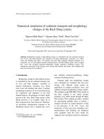
List of Figures

Figure 2.1: Definition sketch of bed elevation, free surface elevation and total water
depth. ………………………………………………………………………………… 22

Figure 2.2: Streamline coordinate system; z-axis points out of paper. ……………… 40

Figure 2.3: Sketch of velocity component profiles and wall shear stress components. 40

Figure 2.4: Polar plot of the triangular model for the velocity components. ……………41

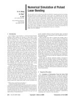
Figure 2.5: Diagram of the drag force and gravitational force component acting on a
sediment particle resting on a sloping bed. ……………………………….………… 46

Figure 2.6: Comparisons between measured and calculated bed load transport rates,
( ): Left: calculated using van Rijn (1984a) equation; Right: calculated using Meyer-
Peter and Muller (1948) equation. …………………………………………… 52
b
q
2
m /s

Figure 2.7: Diagram of the angle relationships among the forces acting on a sediment
particle resting on a sloping bed in case of downslope flow: (a) 3D view; (b) Force
triangle. ………………………………………………………………………………… 56

Figure 2.8: Diagram of the angle relationships among the forces acting on a sediment
particle resting on a sloping bed in case of upslope flow: (a) 3D view; (b) Force
triangle. ……………………………………………………………………………… 57

Figure 3.1: A single cell of the staggered grid and the locations of variables. ……… 66

Figure 4.1: Definition sketch of a solitary wave. ………………………….………… 89

Figure 4.2: (a) Comparisons of the solitary wave profiles at different time
0
/tgh= (A):
125.26, (B): 250.53, (C): 375.79, (D): 501.06 and (E): 626.32 between the analytical
solutions (dashed line) and the numerical results (solid line). (b) Time histories of the
mass (dash-dot line), total energy (solid line), kinetic energy (dashed line) and potential
energy (dotted line); the mass has been normalized by the calculated mass at
0
/ 250.53tgh and the energy has been normalized by the calculated total energy at
0
/ 250.53tgh ………………………………….…….…………………………… 92

Figure 4.3: (a) Comparisons of the solitary wave profiles at time
0
/ =501.06tgh among
the analytical solutions (dashed line), the numerical results using (circles), 4.0 mx

xi
2.0
mx (dotted line), (dash-dot line) and 1.0 mx 0.5mx

 (solid line). (b)
Numerical convergence in terms of the wave height at time
0
/ =501.06tgh ; analytical
solution (dashed line) and the numerical solutions (circles). ………………………… 94

Figure 4.4: Breaking of a dam: (a) at
0

; (b) at
0
tt

. …………………………… 97 t

Figure 4.5: Com
parisons of both water depth and velocity between the analytical solutions
(solid line) and the numerical results (dashed line). Initial water depth before dam-break is
also plotted (dotted line). …………………………………… ……………………… 98

Figure 4.6: Definition sketch of the initial condition of the partial dam-break problem and
the positions of four measurement stations, i.e., STA100, STA150, STA225 and
STA350……………………………………………………………………………… 101

Figure 4.7: Comparisons of both water depth and velocity between the experimental data
(circle) and the numerical results (solid line) at stations STA100, STA150, STA225 and

STA350. ……………………………………………………………………………… 102

Figure 4.8: Numerical results of the water surface profile at different time t=0, 15, 30, 45
and 60 seconds and at final steady state. ……………………………….…………… 105

Figure 4.9: Comparisons of water surface profile between the experimental data (cross)
and the numerical results (solid line). ……………………………………………… 105

Figure 4.10: Comparisons of the time histories of the normalized water surface elevation
(a) at the center

and (b) at the corner



0, 0
nx ny
0
/ H

5m,5m of the tank among the
linear analytical solution (solid line), the numerical results using (dashed
line), (dash-dot line) and
50
100
nynx 200nx ny


(dotted line) ….…………… 109

Figure 4.11: Time histories of the mass (dashed line) and total energy (solid line); the
mass has been normalized by the calculated mass at
t 0

and the energy has been
normalized by the calculated total energy at
0t

. ……………………… …… 110

Figure 4.12: Snap shots of the free surface profiles during the water sloshing at t

(a) 0,
(b) 5 s, (c) 10 s, (d) 15 s, (e) 20 s and (f) 25 s. …………………………………….… 111

Figure 4.13: Comparisons of depth-averaged longitudinal velocities between the
experimental data (x/h=60: square; x/h=100: triangle; x/h=150: circle) and numerical
results. ……………………………………………………………………………… 113

Figure 4.14: Grid arrangement in the computational domain; groyne is located at x=2m;
lines are plotted every two grid nodes for easier visibility. ……………… ……… 117

Figure 4.15: Computed streamline pattern and the recirculating length; x/b=0 is the groyne
position along flume direction. ……………………………………………… 117

xii

Figure 4.16: Com
parisons of the normalized depth-averaged resultant velocity profiles
among the experimental data (circle), the numerical results from the present model (solid

line), from Molls et al. (1995) (dash-dot line) and from Tingsanchali and Maheswaran
(1990) (dotted line); all the velocities are normalized by
0
0.253 m/sU

; /xb 0

is the
groyne position along flume direction. ……………………………………… ……… 118

Figure 4.17: Comparisons of the normalized bed shear stress profiles among the
experimental data (circle), the numerical results from the present model (solid line), from
the present model with the correction of the bed shear stress (dashed line) and from
Tingsanchali and Maheswaran (1990) (dotted line); all the shear stresses are normalized
by measured
in upstream region;
2
0
0.1293 N/m


/xb 0

is the groyne position along
flume direction. ………………………………………………………… ………… 119

Figure 4.18: Comparisons of the concentration distributions between the analytical
solution (solid lines) and the numerical results (dashed lines) at
t=0, 2, 4, 6 and 8s (from
left to right). ………………………………………………………………………… 121

Figure 4.19: Time history of the total volume of the concentration; the total volume of
concentration is normalized by its initial value. …………………………………… 122

Figure 4.20: Three-dimensional perspective view of the initial hump (left) and the hump at
t =1.25 s (right), for the numerical results. ………………………….…………… 124

Figure 4.21: The contours of (a): initial hump and (b): hump at
t=1.25s. Dashed lines:
numerical results; solid lines: analytical solution. ……………………….………… 125

Figure 4.22: Time history of the total volume of the concentration; the total volume of
concentration is normalized by its initial value. …………………………………… 126

Figure 4.23: Three-dimensional perspective view of the concentration distribution at
t=36000s, for the numerical results. ………………………………………………… 128

Figure 4.24: The contour of the concentration distribution at
t=36000s. Dashed line:
numerical results; solid line: analytical solution. ……………………………….…… 129

Figure 4.25: Time history of the total volume of the concentration; the total volume of
concentration is normalized by its initial value. …………………………….……… 130

Figure 4.26: Numerical simulation of Gaussian hump evolution up to 10,000 s. …… 133

Figure 4.27: Comparisons of the bed elevation between the analytical solution (solid line)
and the numerical result (circle) at
t=600 s (left), 2000 s (middle) and 6000 s (right). 134

xiii
Figure 4.28: Tim
e history of the total volume of the sand bed; the total volume of the sand
bed is normalized by its initial total volume. ……………………….………… 135

Figure 5.2: Sketches of the initial trench profiles and locations of measurements for flow
velocity and sediment concentration profiles: (a) Test 1 with measurement locations 1 ~ 8;
(b) Test 2 with measurement positions 1 ~ 5; (c) Test 3 with measurement locations 1 ~ 5.
All dimensions are in meter.
……………………………………………………… 139

Figure 5.2 (a): Flow velocities at positions 1~8 in Test 1. Circle: measured velocity
profiles across water depth; Solid line: depth-averaged values of measured velocity
profiles; Dashed line: numerical results of depth-averaged velocities; Dotted line: depth-
averaged velocities calculated based on flow fluxes; (b): Measurement positions 1~8 in
Test 1. …………………………………………………………………………………. 144

Figure 5.3 (a): Sediment concentrations at positions 1~8 in Test 1. Circle: measured
concentration profiles across water depth; Solid line: depth-averaged values of measured
concentration profiles; Dashed line: numerical results of depth-averaged concentrations;
(b): Measurement positions 1~8 in Test 1. …………………………………………… 145

Figure 5.4 (a): Flow velocities at positions 1~5 in Test 2. Circle: measured velocity
profiles across water depth; Solid line: depth-averaged values of measured velocity
profiles; Dashed line: numerical results of depth-averaged velocities; Dotted line: depth-
averaged velocities calculated based on flow fluxes; (b): Measurement positions 1~5 in
Test 2. ………………………………………………………………… ……………… 146

Figure 5.5 (a): Sediment concentrations at positions 1~5 in Test 2. Circle: measured
concentration profiles across water depth; Solid line: depth-averaged values of measured

concentration profiles; Dashed line: numerical results of depth-averaged concentrations;
(b): Measurement positions 1~5 in Test 2. …………………………………………….147

Figure 5.6 (a): Flow velocities at positions 1~5 in Test 3. Circle: measured velocity
profiles across water depth; Solid line: depth-averaged values of measured velocity
profiles; Dashed line: numerical results of depth-averaged velocities; Dotted line: depth-
averaged velocities calculated based on flow fluxes; (b): Measurement positions 1~5 in
Test 3. ………………………………………………………………………………… 148

Figure 5.7 (a): Sediment concentrations at positions 1~5 in Test 3. Circle: measured
concentration profiles across water depth; Solid line: depth-averaged values of measured
concentration profiles; Dashed line: numerical results of depth-averaged concentrations;
(b): Measurement positions 1~5 in Test 3. ……………………………………………149

Figure 5.8: Comparisons of numerical results of bed elevations at
t=1, 3, 5, …, 13 and
15hr in Test 1 calculated from regular method (dashed line) and from approximate method
(dotted line). Initial trench profile (solid line) and water surface (dash-dot line) are also
shown. ……………………….…………………………………………………………151


xiv
Figure 5.9: Bed elevations at
t=1, 3, 5, …, 13 and 15hr in Test 1 calculated from regular
method versus from approximate method (dots). Solid line: perfect agreement. …… 152

Figure 5.10: Bed elevation comparisons after 7.5 and 15 hours between numerical results
and experimental data in Test 1. Solid line: initial bed; Circles and triangles: bed measured
after 7.5 and 15 hours respectively; Dash-dot and dashed lines: present numerical results
after 7.5 and 15 hours respectively; Lines with plus and with cross: van Rijn’s numerical

results after 7.5 and 15 hours respectively; Dotted line: numerical result of water surface
after 15 hours. …………………………………………………………………………155

Figure 5.11: Bed elevation comparisons after 7.5 and 15 hours between numerical results
and experimental data in Test 2. Solid line: initial bed; Circles and triangles: bed measured
after 7.5 and 15 hours respectively; Dash-dot and dashed lines: present numerical results
after 7.5 and 15 hours respectively; Lines with plus and with cross: van Rijn’s numerical
results after 7.5 and 15 hours respectively; Dotted line: numerical result of water surface
after 15 hours. ……………………………………….……………………………… 156

Figure 5.12: Bed elevation comparisons after 7.5 and 15 hours between numerical results
and experimental data in Test 3. Solid line: initial bed; Circles and triangles: bed measured
after 7.5 and 15 hours respectively; Dash-dot and dashed lines: present numerical results
after 7.5 and 15 hours respectively; Lines with plus and with cross: van Rijn’s numerical
results after 7.5 and 15 hours respectively; Dotted line: numerical result of water surface
after 15 hours. ……………………………………………………….……………… 157

Figure 5.13: Comparisons of bed elevations in Test 1 after 7.5 and 15 hours between
numerical results simulated with and without bed slope effect. Solid line: initial bed
profile; Circles and triangles: experimental measurements of bed elevation after 7.5 and 15
hours respectively; Dash-dot line and dashed line: numerical results of bed elevation after
7.5 and 15 hours from present model with bed slope effect; Line with plus and with cross:
numerical results of bed elevation after 7.5 and 15 hours respectively from present model
without bed slope effect; Dotted line: numerical result of water surface after 15
hours. ………………………………………………………………………………… 159

Figure 5.14: Comparisons of bed elevations in Test 2 after 7.5 and 15 hours between
numerical results simulated with and without bed slope effect. Solid line: initial bed
profile; Circles and triangles: experimental measurements of bed elevation after 7.5 and 15
hours respectively; Dash-dot line and dashed line: numerical results of bed elevation after

7.5 and 15 hours from present model with bed slope effect; Line with plus and with cross:
numerical results of bed elevation after 7.5 and 15 hours respectively from present model
without bed slope effect; Dotted line: numerical result of water surface after 15
hours. ………………………………………………………………………………… 160

Figure 5.15: Comparisons of bed elevations in Test 3 after 7.5 and 15 hours between
numerical results simulated with and without bed slope eff
ect. Solid line: initial bed
profile; Circles and triangles: experimental measurements of bed elevation after 7.5 and 15
hours respectively; Dash-dot line and dashed line: numerical results of bed elevation after
7.5 and 15 hours from present model with bed slope effect; Line with plus and with cross:

xv
num
erical results of bed elevation after 7.5 and 15 hours respectively from present model
without bed slope effect; Dotted line: numerical result of water surface after 15
hours. …………………………………………………………………………………161

Figure 5.16: Comparison of bed elevations after 7.5 and 15 hours in Test 3 predicted using
different values of angle of repose. Solid line: initial bed profile; Circles and triangles:
experimental measurements of bed elevation after 7.5 and 15 hours respectively; Dash-dot
line: bed elevations after 7.5 and 15 hours using ; Dashed line: bed elevations after
7.5 and 15 hours using ; Line with plus: bed elevations after 7.5 and 15 hours using
; Dotted line: numerical result of water surface after 15 hours. ……………….163
27



31




35




Figure 5.37: Sketch of initial dune profile. All dim
ensions are in meter. ……………165

Figure 5.18: Particle size distribution curves of three sand samples. ………………….165

Figure 5.19: Bed elevations of 1D dune measured at (a):
t=0.5hr; (b): t=1hr; (c): t=1.5hr;
and (d):
t=2hr in Test 1 (solid line), Test 2 (dashed line) and Test 3 (dash-dot line). Dotted
line: initial profile. ……………………………………………………… ………… 168

Figure 5.20: Averaged bed elevations of Test 1, 2 and 3 at
t=0.5hr (solid line), 1hr (dashed
line), 1.5hr (dash-dot line) and 2hr (crosses). Dotted line: initial profile. …………….168

Figure 5.21: Comparisons of bed elevations of the dune at
t=0, 0.5, 1, 1.5 and 2 hours
between numerical results (solid line) and experimental data (dashed line). ………….170

Figure 5.22: Time history of total volume of sand dune; total volume of the sand dune is
normalized by its initial total volume. …………………………………………………171

Figure 5.23: Comparisons of bed elevations at

t=0, 0.5, 1, 1.5 and 2 hours between
numerical results simulated with (solid line) and without (dash-dot line) bed slope effect.
Dashed line: measured bed elevations. ……………………………………………… 172

Figure 5.24: Comparisons of bed elevations at
t=0, 0.5, 1, 1.5 and 2 hours predicted using
different values of angle of repose. Solid line: numerical results using ; Dash-dot
line: num
erical results using ; Dotted line: numerical results using ; Dashed
li
ne: measured bed elevations. ……………………………………………………… 173
27



35


31


 

Figure 6.4: Plan view sketch of channel w
ith suddenly-expanded cross-section;
x=0 is
expansion position. Dots represent horizontal locations of velocity measurement. …178

Figure 6.5: Time series of velocity components (a):
u, (b): v and (c): w at location (-10cm,

45cm, 5cm). ……………………………………………………………………………185

Figure 6.6: Wave number spectra of total kinetic energy at location (-10cm, 45cm, 5cm)
and the inertial subrange. ………………………………………………………………186

xvi

Figure 6.7: Computational dom
ain and grid arrangement in sudden-expanded channel;
lines are plotted every two grid nodes for easier visibility. ……………………………187

Figure 6.8: Depth-averaged velocity
U
(Crosses: experimental data; Solid lines:
numerical results);
U
is normalized by
0
0.53 m/sU

; x=0 is the expansion
position. ………………………………………………………………………………189

Figure 6.9: Depth-averaged velocity
V (Crosses and pluses: experimental data; Solid lines:
numerical results);
V is normalized by
0
0.53 m/sU


; x=0 is the expansion
position. ……………………………………………………………………………… 190

Figure 6.10: Depth-averaged TKE (Crosses: experimental data; Solid lines: numerical
results); is normalized by ; x=0 is the expansion position. ………… …………191

ˆ
k
ˆ
k
2
0
U

Figure 6.11: Depth-averaged dissipation rate
ˆ

(Crosses: experimental data: Solid lines:
numerical results);
ˆ

is normalized by ; x=0 is the expansion position. ………192
3
0
/U
0
H

Figure 6.12: Depth-averaged turbulent viscosity
ˆ

t

(Crosses: experimental data: Solid
lines: numerical results);
ˆ
t

is normalized by ; x=0 is the expansion
position. ……… 193
00
UH

Figure 6.13: Measurem
ents of bed profiles along
y=5, 10, …, 50 and 55 cm at (a) t=1 hr;
(b)
t=2 hr; (c) t=3 hr; (d) t=4 hr; (e) t=5 hr; (f) t=6 hr; (g) t=7 hr; and (h) t=8 hr in Test 1, 2
and 3;
x=0 is at the abrupt expansion. …………………………………….…………….197

Figure 6.14: Contour of bed elevations at: (a)
t=1 hr; (b) t=2 hr(c) t=3 hr; (d) t=4 hr; (e)
t=5 hr; (f) t=6 hr; (g) t=7 hr; and (h) t=8 hr. Upper panel: averaged values of
measurements from three tests; lower panel: numerical results. …………… …………206

Figure 6.15: Plan view sketch of channel with suddenly-contracted cross-section;
x=0 is
contraction position. Dots represent locations of velocity measurement. ………… 212

Figure 6.16: Computational domain and grid arrangement in sudden-contracted channel;

lines are plotted every two grid nodes for easier visibility. ……………………………213

Figure 6.17: Depth-averaged velocity
U (Crosses: experimental data; Solid lines:
numerical results);
U is normalized by
0
0.2 m/sU

; x=0 is at the abrupt
contraction. ……………………………………………………………………………216

Figure 6.18: Depth-averaged velocity
V (Crosses: experimental data; Solid lines:
numerical results);
V
is normalized by
0
0.2 m/sU

; x=0 is at the abrupt
contraction. ……………………………………………………………………………217

xvii
Figure 6.19: Depth-averaged TKE (Crosses: experimental data; Solid lines: numerical
results); is normalized by ;
x=0 is at the abrupt contraction. ……………………218
ˆ
k
ˆ

k
2
0
U

Figure 6.20: Depth-averaged dissipation rate
ˆ

(Crosses: experimental data: Solid lines:
numerical results);
ˆ

is normalized by ; x=0 is at the abrupt contraction. ……219
3
0
/U
0
H

Figure 6.21: Depth-averaged turbulent viscosity
ˆ
t

(Crosses: experimental data: Solid
lines: numerical results);
ˆ
t

is normalized by ; x=0 is at the abrupt
contraction. ……………………………………………………………………………220

00
UH

Figure 6.22: Measurements of bed heights along y=5, 10, …, 50 and 55 cm at t=2 hours in
Test 1, 2 and 3; x=0 is contraction position. ………………………………………222

Figure 6.23: Contour of bed elevations at: (a) t=0.5hr; (b) t=1hr; (c) t=1.5hr; and (d) t=2hr.
Upper panel: averaged values of measurements from three tests; lower panel: numerical
results with correction for bed shear stress. ………………………………224

Figure 6.24: Comparisons of bed elevations among experimental measurements,
numerical results with and without correction for bed shear stress at: (a) t=0.5hr; (b) t=1hr;
(c) t=1.5hr; and (d) t=2hr. x=0 is contraction position. …………………………………230

Figure 6.25: Plan view sketch of channel consisting of a contraction and an expansion.
Dots represent horizontal locations of velocity measurement (Duc and Rodi, 2008). All
dimensions are in meter. ……………………………………………………………… 235

Figure 6.26: Resultant velocity field in Run 1: (a) Depth-averaged velocity field calculated
using the present model; (b) Velocity field at free surface calculated using FAST3D (Duc
and Rodi, 2008); (c) Measured velocity field at free surface (Duc and Rodi, 2008).
Velocities are in m/s. ……………………………………………………………………239

Figure 6.27: Depth-averaged resultant velocities. Solid lines: numerical results calculated
using present model; Crosses: numerical results calculated using FAST3D (Duc and Rodi,
2008); Circles: experimental measurements (Duc and Rodi, 2008). Velocities are in
m/s. ……………………………………………………………………………………240

Figure 6.28: Comparisons of water surface along centerline of contracted channel
(y=0.25m) among experimental measurements (circles; Duc and Rodi, 2008), numerical

results using present model (solid line) and numerical results using FAST3D (dashed line;
Duc and Rodi, 2008). ……………… ………………………………………………….240

Figure 6.29: Contour of bed elevations at the end of Run 3 (at t=125 min): (a) Numerical
results using present model; (b) Numerical results using FAST3D (Duc and Rodi, 2008);
(c) Experimental measurements (Duc and Rodi, 2008). Bed elevations are in m
eter. …243


xviii

xix
Figure 6.30: Comparisons of bed elevations along centerline of contracted channel
(y=0.25m) at the end of Run 3 (at t=125 min) among experimental measurements (circles;
Duc and Rodi, 2008), numerical results using present model (solid line) and using
FAST3D (dashed line; Duc and Rodi, 2008). ……………….………………………….244

Figure 6.31: Comparisons of water surface along centerline of contracted channel
(y=0.25m) at the end of Run 3 (at t=125 min) among experimental measurements (circles;
Duc and Rodi, 2008), numerical results using present model (solid line) and using
FAST3D (dashed line; Duc and Rodi, 2008). ………….……………………………….245




List of Symbols

a
reference level
1/2i

a

Roe speed of bed-form propagation
A
parameter
B
channel width
c sediment concentration
C depth-averaged sediment concentration
a
C reference concentration at reference level a
ea
C
,
equilibrium near-bed concentration
b
C depth-averaged bed-load concentration
D
C drag force coefficient
wave
C wave celerity
f
c friction coefficient
f
x
c
friction coefficient in x-direction
k
c , empirical constants


c

C , , empirical constants in turbulence model

1
C

2
C

b
zC bed-form propagation phase speed
Flow
Cr , Courant numbers for flow and suspended load computations
Sedi
Cr
d
sediment particle diameter
50
d median diameter of the sediment particle

xx
10
d , sediment particle diameter such that 10% and 90% of all the grain
sizes are smaller than and , respectively
90
d
10
d
90

d
sphere
d diameter of the sphere
*
D particle size parameter
D
F drag force
,0cr
F drag force for sediment particle on a flat bed
,cr
F

drag force for sediment particle on a slope
Fr Froude number
ˆ
F
kX
,
ˆ
F
kY
convection terms in
ˆ
k

equation
ˆ
FX

,

ˆ
FY

convection terms in
ˆ


equations
CX
F , sediment fluxes in x- and y-directions
CY
F
i
g i-th component of the gravitational acceleration
H
water depth
f
H
flooding depth
,
ij spatial nodes when subscript
k turbulent kinetic energy
k
ˆ
depth-averaged turbulent kinetic energy
k

wave number
s
k Nikuradse roughness

12
,kk correction factors for streamwise and transverse sloping beds
n Manning’s roughness coefficient; time level when superscript

xxi
,nx ny grid numbers in x- and y-directions
p
pressure
,PQ volume flux components in x- and y-directions
P production of turbulent kinetic energy
n
P , flow flux components normal and tangential to the solid boundary

P
h
P horizontal production term of turbulent kinetic energy
kV
P , vertical production terms of turbulent kinetic energy and its
dissipation rate
V
P

p
oro porosity factor of sediment
b
q bed load transport rate
,
bx by
qq bed load transport rates in x- and y-directions
R

resultant force of the drag force and gravitational force component
along the steepest slope
R
e Reynolds number
*
R
e grain Reynolds number
S energy slope
s
specific gravity of the particle
D
S , sediment deposition and entrainment fluxes
E
S
t time
T excess bed shear stress parameter
x
x
T , ,
yx
T
x
y
T , depth-averaged effective stresses
yy
T
,,
uvw velocity components in x-, y- and z-directions

xxii

,,uvw mean velocities in x-, y- and z-directions
', ', '
uvw velocity fluctuations in x-, y- and z-directions
U
,
V
depth-averaged velocity components in x- and y-directions
max
U , maximum depth-averaged velocities in x- and y-directions
max
V
main
U main stream velocity
R
U resultant velocity
U

tangential velocity
*
u friction velocity
f
u velocity in a hypothetical two-dimensional boundary layer
ˆ
VISkX , diffusion terms in
ˆ
VISkY
ˆ
k

equation

ˆ
VIS X

,
ˆ
VIS Y

diffusion terms in
ˆ


equations
f
w settling velocity of sediment particle
,,
x
yz coordinates in Cartesian coordinate system
W submerged weight of sediment particle
0
y
zero-velocity level in the logarithmic law-of-the-wall
b
z bed elevation which is reckoned negative when measured vertically
upwards with respect to the datum

angle between flow and x-axis

slope angle
x


,
y

angles that the slope makes with x- and y-axes

xxiii