Robust identification and controller design for delay processes

ROBUST IDENTIFICATION AND
CONTROLLER DESIGN FOR DELAY
PROCESSES
LIU MIN
NATIONAL UNIVERSITY OF SINGAPORE
2007
Founded 1905
ROBUST IDENTIFICATION AND
CONTROLLER DESIGN FOR DELAY
PROCESSES
BY
LIU MIN (B.ENG., M.ENG.)
DEPARTMENT OF ELECTRICAL AND COMPUTER
ENGINEERING
A THESIS SUBMITTED
FOR THE DEGREE OF DOCTOR OF PHILOSOPHY
NATIONAL UNIVERSITY OF SINGAPORE
2007
Acknowledgments
I would like to express my sincere appreciation to my supervisor, Professor Wang,
Qing-Guo, for his excellent guidance and gracious encouragement through my
study. His uncompromising research attitude and stimulating advice helped me
in overcoming obstacles in my research. His wealth of knowledge and accurate
foresight benefited me in finding the new ideas. Without him, I would not be able
to finish the work here. I would also like to express my sincere appreciation to my
supervisor, Professor Hang Chang Chieh, for his constructive suggestions which
benefited my research a lot. I have learnt much from them over the years both
academically and intellectually. To both of them, my most sincere thanks.
I would also like to express my thanks to Dr. Zhang Yong, Dr. Yang Xue-ping
and Dr. Bi Qiang for their comments, advice, and inspiration. Special gratitude
goes to my friends and colleagues. I would like to express my thanks to Dr. He

Yong, Dr. Fu Jun, Dr. Lu Xiang, Dr. Ye Zhen, Dr. Zhou Hanqing, Mr. Li Heng,
Mr. Zhang Zhiping and many others working in the Advanced Control Technology
Lab. I enjoyed very much the time spent with them.
Finally, this thesis would not be finished without the love and support of my
wife, Qin Meng. Thank you very much. The encouragement and love from my
parents are invaluable to me. I would like to devote this thesis to them all.
i
Contents
Acknowledgements i
List of Figures vi
List of Tables vii
Summary viii
1 Introduction 1
1.1 Motivation . . . . . . . . . . . . . . . . . . . . . . . . . . . . . . . . 1
1.2 Contributions . . . . . . . . . . . . . . . . . . . . . . . . . . . . . . 7
1.3 Organization of the thesis . . . . . . . . . . . . . . . . . . . . . . . 9
2 Process Identification from Pulse Tests 10
2.1 Introduction . . . . . . . . . . . . . . . . . . . . . . . . . . . . . . . 10
2.2 Identification from pulse tests . . . . . . . . . . . . . . . . . . . . . 11
2.3 Simulation . . . . . . . . . . . . . . . . . . . . . . . . . . . . . . . . 16
2.4 Real time testing . . . . . . . . . . . . . . . . . . . . . . . . . . . . 20
2.5 Conclusion . . . . . . . . . . . . . . . . . . . . . . . . . . . . . . . . 20
3 Process Identification from Step Tests 22
3.1 Introduction . . . . . . . . . . . . . . . . . . . . . . . . . . . . . . . 22
3.2 Review of integral identification . . . . . . . . . . . . . . . . . . . . 23
3.3 The proposed method . . . . . . . . . . . . . . . . . . . . . . . . . 25
3.4 High-order modelling from step tests . . . . . . . . . . . . . . . . . 31
ii
Contents iii
3.5 Real time testing . . . . . . . . . . . . . . . . . . . . . . . . . . . . 34

3.6 Conclusions . . . . . . . . . . . . . . . . . . . . . . . . . . . . . . . 36
4 Process Identification from Relay Tests 38
4.1 Introduction . . . . . . . . . . . . . . . . . . . . . . . . . . . . . . . 38
4.2 FFT method revisited . . . . . . . . . . . . . . . . . . . . . . . . . 39
4.3 First-order modelling . . . . . . . . . . . . . . . . . . . . . . . . . . 43
4.4 n-th order modelling . . . . . . . . . . . . . . . . . . . . . . . . . . 52
4.5 Conclusion . . . . . . . . . . . . . . . . . . . . . . . . . . . . . . . . 57
5 Process Identification from Piecewise Step Tests 58
5.1 Introduction . . . . . . . . . . . . . . . . . . . . . . . . . . . . . . . 58
5.2 Second-order modelling . . . . . . . . . . . . . . . . . . . . . . . . . 59
5.3 n-th order modelling . . . . . . . . . . . . . . . . . . . . . . . . . . 67
5.4 Conclusion . . . . . . . . . . . . . . . . . . . . . . . . . . . . . . . . 70
6 Multivariable Process Identification 71
6.1 Introduction . . . . . . . . . . . . . . . . . . . . . . . . . . . . . . . 71
6.2 TITO processes . . . . . . . . . . . . . . . . . . . . . . . . . . . . . 72
6.3 Simulation studies . . . . . . . . . . . . . . . . . . . . . . . . . . . 78
6.4 General MIMO processes . . . . . . . . . . . . . . . . . . . . . . . . 84
6.5 Real time testing . . . . . . . . . . . . . . . . . . . . . . . . . . . . 90
6.6 Conclusion . . . . . . . . . . . . . . . . . . . . . . . . . . . . . . . . 91
7 PID Controller Design by Approximate Pole Placement 93
7.1 Introduction . . . . . . . . . . . . . . . . . . . . . . . . . . . . . . . 93
7.2 Problem statement . . . . . . . . . . . . . . . . . . . . . . . . . . . 95
7.3 The proposed method . . . . . . . . . . . . . . . . . . . . . . . . . 97
7.4 Simulation study . . . . . . . . . . . . . . . . . . . . . . . . . . . . 99
7.5 Real time testing . . . . . . . . . . . . . . . . . . . . . . . . . . . . 107
7.6 Positive PID settings . . . . . . . . . . . . . . . . . . . . . . . . . . 107
7.7 Oscillation processes . . . . . . . . . . . . . . . . . . . . . . . . . . 109
Contents iv
7.8 Multivariable case . . . . . . . . . . . . . . . . . . . . . . . . . . . . 114
7.9 Conclusion . . . . . . . . . . . . . . . . . . . . . . . . . . . . . . . . 120

8 Conclusions 122
8.1 Main findings . . . . . . . . . . . . . . . . . . . . . . . . . . . . . . 122
8.2 Suggestions for further work . . . . . . . . . . . . . . . . . . . . . . 124
Bibliography 126
Author’s Publications 134
List of Figures
2.1 Rectangular pulse response and input. . . . . . . . . . . . . . . . . 12
2.2 Rectangular pulse response and input for Example 2.1. . . . . . . . 16
2.3 Rectangular doublet pulse response and input for Example 2.1. . . . 18
2.4 Nyquist curves for Example 2.2. . . . . . . . . . . . . . . . . . . . 18
2.5 DC motor set. . . . . . . . . . . . . . . . . . . . . . . . . . . . . . 20
2.6 Pulse response of the DC motor. . . . . . . . . . . . . . . . . . . . 21
3.1 Step response and input for Example 3.1. . . . . . . . . . . . . . . 29
3.2 Nyquist plot for Example 3.1. . . . . . . . . . . . . . . . . . . . . . 30
3.3 Nyquist plot for Example 3.2. . . . . . . . . . . . . . . . . . . . . . 34
3.4 Step responses and input of the temperature control system. . . . . 35
3.5 Flowchart of the mixing procedure. . . . . . . . . . . . . . . . . . . 36
3.6 Step test of the flow control system. . . . . . . . . . . . . . . . . . . 37
4.1 Relay feedback system. . . . . . . . . . . . . . . . . . . . . . . . . . 40
4.2 Relay function. . . . . . . . . . . . . . . . . . . . . . . . . . . . . . 40
4.3 Process output and input of relay experiment for Example 4.1. . . . 44
4.4 Process output and input of relay experiment. . . . . . . . . . . . . 46
4.5 Process output and input of relay experiment for Example 4.2. . . . 50
4.6 Process output and input of relay experiment for Example 4.3. . . . 51
5.1 Process output and input of relay experiment for Example 5.1. . . . 64
5.2 Pulse response and input for Example 5.1. . . . . . . . . . . . . . . 65
6.1 Identification test of Example 6.1. . . . . . . . . . . . . . . . . . . . 79
v
List of Figures vi
6.2 Calculation of T. . . . . . . . . . . . . . . . . . . . . . . . . . . . . 79

6.3 Relay feedback experiment. . . . . . . . . . . . . . . . . . . . . . . 85
6.4 Identification test of Example 6.2. . . . . . . . . . . . . . . . . . . . 85
6.5 Identification test of Example 6.3. . . . . . . . . . . . . . . . . . . . 89
6.6 Temperature chamber set. . . . . . . . . . . . . . . . . . . . . . . . 91
6.7 Process responses and inputs of the thermal control system. . . . . 92
7.1 PID control systems. . . . . . . . . . . . . . . . . . . . . . . . . . . 96
7.2 Step response and manipulated variable of Example 7.1 with L = 0.5.100
7.3 Step response of Example 7.1 with L = 0.5. . . . . . . . . . . . . . 100
7.4 Step response and manipulated variable of Example 7.1 with L = 2. 102
7.5 Step response of Example 7.1 with L = 2. . . . . . . . . . . . . . . 102
7.6 Step response and manipulated variable of Example 7.1 with L = 4. 103
7.7 Step response of Example 7.1 with L = 4. . . . . . . . . . . . . . . 103
7.8 Step response and manipulated variable of Example 7.2. . . . . . . 105
7.9 Step response of Example 7.2. . . . . . . . . . . . . . . . . . . . . . 106
7.10 Step response, measured response and manipulated variable of Ex-
ample 7.2. . . . . . . . . . . . . . . . . . . . . . . . . . . . . . . . . 106
7.11 Step response and manipulated variable of the thermal chamber. . . 108
7.12 Step response and manipulated variable of Example 7.1 with L = 0.5.110
7.13 Step response of Example 7.1 with L = 0.5. . . . . . . . . . . . . . 110
7.14 Step response and manipulated variable of Example 7.3. . . . . . . 113
7.15 Step response of Example 7.3. . . . . . . . . . . . . . . . . . . . . . 113
7.16 Step response and manipulated variable of Example 7.4. . . . . . . 114
7.17 Step response of Example 7.4. . . . . . . . . . . . . . . . . . . . . . 115
7.18 Step response of Example 7.5. . . . . . . . . . . . . . . . . . . . . . 117
7.19 Step response of Example 7.6. . . . . . . . . . . . . . . . . . . . . . 119
7.20 Step response of Example 7.7. . . . . . . . . . . . . . . . . . . . . 121
List of Tables
2.1 Identification results for Example 2.3 . . . . . . . . . . . . . . . . . 19
3.1 Identification results for Example 3.1 . . . . . . . . . . . . . . . . . 31
4.1 Identification errors for Example 4.1 . . . . . . . . . . . . . . . . . . 44

4.2 Identification errors for Example 4.2 . . . . . . . . . . . . . . . . . . 50
4.3 Identification errors for Example 4.3 . . . . . . . . . . . . . . . . . . 56
4.4 Identification errors for Example 4.4 . . . . . . . . . . . . . . . . . . 57
5.1 Identification results for different second order processes . . . . . . 66
6.1 Estimated model parameters of Example 6.1 . . . . . . . . . . . . . 83
vii
Summary
Process identification plays an important role in process analysis, controller design,
system optimization and fault detection. One of the active and difficult areas in
process identification is in time delay systems. Time delay exists in many indus-
trial processes and has a significant effect on the performance of control systems.
Thus, identification of unknown time delay needs special attention. In this thesis,
a series of identification methods are proposed for continuous-time delay processes.
Both open-loop identification tests and closed-loop ones are considered. The initial
conditions are unknown and can be nonzero. The disturbance can be a static or dy-
namic one. Regression equations are derived according to types of test signals. All
the parameters including time delay are estimated without iteration. These identi-
fication methods show great robustness against noise in output measurements but
require no filtering of noisy data.
In the context of pulse tests, a two-stage integral identification method is pre-
sented for continuous-time delay processes. It is noticed that the output response
from a pulse test will still be significant and last for a long time after the pulse dis-
appears. We take advantage of this feature. The integral intervals are specifically
chosen and this enables easy and decoupled identification of the system parameters
in two stages.
In the context of step tests, a one-stage integral identification method is devel-
oped for continuous-time delay processes. The key idea is to make both upper and
lower limits of the inner integral dependent of the dummy variable of the outer in-
viii
Summary ix

tegral so that the initial conditions do not appear in the resulting integral equation.
In the context of relay tests, the fast Fourier transform based identification
method is revisited first and the need for further development is discussed. An
identification method from relay tests is proposed. By viewing a relay test as a
sequence of step tests, the integral technique is adopted to devise the algorithm.
A general integral identification method is then proposed. The identification test
can be of open-loop type such as pseudo random binary signals and pulse tests,
or of closed-lo op type such as relay tests. The disturbance can be of general form.
The proposed new regression equation has more linearly independent functions and
thus enables to identify a full process model with time delay as well as combined
effects of unknown initial condition and disturbance without any iteration.
Most industrial processes are of multivariable in nature and time delay is present
in most industrial processes. Identification of multivariable processes with multiple
time delay is in great demand. To this end, an effective identification technique is
presented for multivariable delay processes. The technique covers all popular tests
used in applications, requires reasonable amount of computations, and provides
accurate and robust identification results.
The model obtained from process identification may be used for controller de-
sign. In the thesis, an analytical PID design method is proposed for continuous-
time delay systems to achieve approximate pole placement with dominance. It
is well known that a continuous-time feedback system with time delay has infi-
nite spectrum and it is impossible to assign such infinite spectrum with a finite-
dimensional controller. In such a case, only the partial pole placement may be
feasible and hopefully some of the assigned poles are dominant. But there is no
easy way to guarantee dominance of the desired poles. The idea presented is to
bypass continuous infinite spectrum problems by converting a delay process to a
rational discrete model and getting back continuous PID controller from its dis-
Summary x
crete form designed for the model with pole placement.
As shown in the given simulation examples and real time tests, the findings can

be applied to industrial control systems. The schemes and results presented in this
thesis have both theoretical contributions and practical values.
Chapter 1
Introduction
1.1 Motivation
The need for process model arises from various engineering tasks such as pro-
cess design, process control, plant optimization and fault detection (Ikonen and
Najin, 2002). Identification is the experimental approach to process modeling
(
˚
Astr¨om and Wittenmark, 1990) and has been an active area in control engineering
(Soderstrom and Mossberg, 2000). Many text books and book chapters have been
published on identification, for examples, Soderstrom and Stoica (1983), Ljung
(1987), Unbehauen and Rao (1987), Sinha and Rao (1991), Johansson (1993) and
Ikonen and Najin (2002). It is also a hot topic in international academic journals
and many publications are available on this topic, see the following special issues:
Automatica 1981 v.17(1), Automatica 1990 v.26(1), IEEEAC 1992 v.37(7), Au-
tomatica 1995 v.31(12), Journal of Process Control 1995 v.5(2) and Automatica
2005 v.41(3).
System identification involves three components: test design, model structure
identification and parameter estimation (Ljung, 1999). A specific test is designed
and input and output responses during such a test will be then recorded. The
model structure and parameter are then identified. The objective of test design is
to excite the process sufficiently to enable identification of the process. A model
1
Chapter 1. Introduction 2
with unknown parameters needs to be constructed. Various model structures are
available to assist in modeling a system. The choice of model structures is based
upon understanding of identification method and insight into identification test.
Parameter estimation is employed to determine the unknown model parameters

from recorded data set.
Identification tests are generally divided into open-loop tests and closed-loop
tests. Step tests and pulse tests are the most popular open-loop tests for their
simplicity (Luyben, 1973). They have their own merits. Step tests are the most
simple and dominant ones. Pulse tests return input and output to the original
stead-state and cause less perturbation to process operation. Though there are
many successful applications of open-loop identification, closed-loop identification
is also an important practical issue (Landau and Karimi, 1999). The most popular
closed-loop identification test is relay feedback (
˚
Astr¨om and Hagglund, 1984).
Identification models are generally classified into parametric models and non-
parametric ones (Wellstead, 1981). Frequency response is a kind of nonparametric
model of processes. It is very useful for system analysis, such as Nyquist stability
studies, controller designs (Goodwin et al., 2001) and parametric model building
(Ljung and Glover, 1981). Parametric models are also preferred by many control
engineers (Unbehauen and Rao, 1987; Ninness, 1996; Ljung, 1985; Ljung, 1999),
because most of advanced control strategies are developed based on parametric
models (Morari and Zafiriou, 1989;
˚
Astr¨om and Wittenmark, 1995; Narendra and
Annaswamy, 1989; Anderson and Moore, 1990; Zhou, 1998).
For nonparametric modeling, relay feedback is one of the popular tests because
frequency responses of processes can be obtained from relay tests. In the early
stage of study on relay identifications, only stationary response of a relay test was
used to estimate the process frequency at the oscillation frequency (
˚
Astr¨om and
Hagglund, 1995). Later, an improvement was reported by Wang et al. (1997a).
Chapter 1. Introduction 3

They use a biased relay feedback and can obtain two accurate process frequency
points from one test. These two estimated frequency points can be converted easily
to an first-order plus time delay (FOPTD) model of the process. A lot of chemi-
cal processes can be modelled by using this method. Another modification of the
standard relay was proposed by Bi et al. (1997): a parasitic relay is added to the
standard relay. This method can identify multiple points on the process frequency
response. Recently, relay identification based on fast Fourier transform (FFT) was
developed. It was first shown in Hang et al. (1995) that multiple points on the
process frequency response can be obtained in a step test by applying FFT. This
method has been further improved and used to identify multiple points simulta-
neously from standard relay tests (Wang et al., 1997b). Wang and his colleagues
introduced a decay exponential to rescale the input and output, then applied FFT
to obtain multiple points on the process frequency response. In Wang et al. (1999),
a modified method was developed. Low-pass filters are included in the control loop
and more robust identifications can be obtained. However, these FFT based iden-
tification methods assume that the relay test starts from a steady state and there
is no disturbance during the test. Besides, additional low-pass filters have to be
used to overcome the effect of the measurement noise. These restrictions can limit
their applications in some cases. It is desirable to remove these assumptions for
wider applications.
Among identification methods of parametric models, continuous-time identifi-
cation has been an active area for its advantages in retaining the models of actually
time-continuous dynamic systems in continuous-time domain (Sinha and Lastman,
1982; Saha and Rao, 1983; Unbehauen and Rao, 1987; Sagara and Zhao, 1990). An
important issue with identification of continuous-time parametric models is iden-
tification of time delay (Wang and Gawthrop, 2001; Garnier et al., 2003). Time
delay is a property of physical systems, by which response to the system input
is delayed in its effect (Shinskey, 1976). It exists in many industrial processes.
In most situations time delay is unknown. Because time delay has a significant
Chapter 1. Introduction 4

effect on the performance of the control systems, its estimation needs special at-
tention (Gawthrop, 1984). Many existing identification methods do not consider
time delay or assume known delay because time delay appears nonlinearly in the
regression equation. For these reasons, there are continuing interests in identifica-
tions of delay processes. Some early methods estimate time delay with numerator
polynomial or transfer function. In Kurz and Goedecke (1981), a shift operator
model with expanded numerator polynomial is used to deal with unknown time
delays. Rational transfer functions, such as polynomial approximation and Pade
approximation, are used to estimate time delay in Gawthrop and Nihtila (1985)
and Souza et al. (1988), respectively. These methods proposed in the early days
increase the order of the models and have to identify more model parameters.
Later, a trial and error method was proposed. Elnaggar et al. (1989) assumes a
known delay and then estimates the other transfer function parameters. With the
estimated model, the estimated error is calculated. From all the obtained models,
the one which minimizes the estimated error is chosen as the identification result.
In Ferretti et al. (1991), an algorithm was proposed to recursively update the value
of a small delay by inspection of the phase contribution of the real negative zero
arising in the corresponding sampled system. This method is inefficient. In Mamat
and Fleming (1995) and Rangaiah and Krishnaswamy (1996), graphical methods
were proposed to identify low order models for continuous-time delay system. How-
ever, their methods cannot identify high-order processes and non-minimum-phase
systems and may lead to large estimation errors when noise is considerable.
Recently, new integration identification methods were reported for identifi-
cations of continuous-time delay systems (Wang and Zhang, 2001; Hwang and
Lai, 2004). Integration identification is a branch of linear filter identification
(Unbehauen and Rao, 1987; Rao and Unbehauen, 2006; Garnier et al., 2003). Like
other continuous-time identification methods, integration identification methods
consist of two main parts: signal processing (multiple integration) and parameter
estimation. The multiple integration works as a pre-filter to overcome the noise ef-
Chapter 1. Introduction 5

fect (Unbehauen and Rao, 1990) like analog pre-filter (Young and Jakeman, 1981).
Integration approach for parameter estimation was first proposed by Diamessis
(1965). Later an improvement was made by treating the initial states of the sys-
tem as additional system parameters to be estimated (Mathew and Fairman, 1974).
By then, the effect of the disturbance had not been considered. With the devel-
opment of computer technologies, numerical integration is then used (Whitfield
and Messali, 1987). In Whitfield and Messali (1987), the effect of deterministic
disturbances at system input and output is also included in the analysis. A similar
integral-equation approach has been derived by Golubev and Wang (1982) from
a frequency-domain error criterion. From their works, efficiency and robustness
of integral equation methods have been shown. It was Wang and Zhang (2001)
who first proposed to apply integration method to identify continuous-time delay
systems from step tests without iterations. Their method takes advantage of the
simple nature of step input and a linear regression equation with a new param-
eterization is devised. The least-squares method is then applied to identify the
regression parameters, from which the full model parameters including time delay
are recovered. This method is so robust that the identification results are still
satisfactory without filtering of the measured output, which is corrupted by noise.
However, like FFT methods from relay tests, Wang’s integration method requires
that the tests start from zero initial conditions and there is no disturbance during
the test. Hwang and Lai (2004) proposed a two-stage identification algorithm,
which uses pulse signals as the input. Two regression equations are obtained from
the two edges of the pulse signal, respectively. Then the estimation and/or the
elimination of the initial conditions and disturbances become possible. Their re-
gression parameter vectors involve all parameters together in each of two stages,
and some of them are very complicated functions of process parameters and ini-
tial conditions. This method fails to work in the step test case, the most popular
one in process control applications, because a step test only has one change of its
magnitude. Simplified general identification methods are needed to identify delay
processes under unknown initial conditions and disturbance from popular identifi-

Chapter 1. Introduction 6
cation tests.
Most industrial processes are of multivariable in nature (Ogunnaike and Ray,
1994; Maciejowski, 1989). To achieve performance requirements by using advanced
controller design methods, models of multivaribale processes are needed (Sinha and
Lastman, 1982; Zhu and Backx, 1993; Ikonen and Najin, 2002; Gevers et al., 2006).
To this end, many methods have been proposed to identify multivariable processes,
for examples, methods proposed in Whitfield and Messali (1987), Wang et al.
(2001b) and Garnier et al. (2007). But only a few of them consider time delays.
In Garnier et al. (2007), a model with input delays is considered but these time
delays are supposed to be known. In Wang et al. (2001b), relay tests are applied.
The frequency responses from the inputs to the outputs are obtained by applying
the FFT. The process step response is constructed by using the inverse FFT to
each process channel. Integral identification methods are then used to recover all
the process model parameters including time delay. Their method is very robust
in face of noise. However, their identification methods and those used in Wang et
al. (2003) require zero initial conditions and no significant disturbance. For easy
applications, these assumptions should be removed. Developing a general identifi-
cation method for multivariable delay processes is of great interest and value.
Control design is a key topic of control engineering. It is also one usage
of process identification (Hjalmarsson, 2005). Since the proportional-integral-
derivative(PID) controller was proposed, its tuning has been an attractive area
because PID control offers the simplest and most effective solution to many con-
trol problems (Ang et al., 2005). According to Yamamoto and Hashimoto (1991),
a large number of PID controllers are used in industry and some of them are not
well tuned. To improve this situation, many methods haven been proposed, such
as methods proposed in Persson and
˚
Astr¨om (1993), Ho et al. (1995), Maffezzoni
(1997), Tan et al. (1999), Mattei (2001), Wang et al. (2001a), Zheng et al. (2002b)

and Zheng et al. (2002a). Among them, one important branch is the dominant
Chapter 1. Introduction 7
pole placement. Tuning of PID controllers with dominant closed-loop poles was
first introduced by Persson and
˚
Astr¨om (1993) and further explained in
˚
Astr¨om
and Hagglund (1995). Both methods are based on a simplified model of processes
and thus cannot guarantee the chosen poles to be indeed dominant in reality. In
the case of high-order systems or systems with time delay, these conventional dom-
inant pole designs, if not well handled, could result in sluggish response or even
instability of the closed-loop. Thus it is desirable to have a method to make the
chosen poles dominant by using PID controller.
1.2 Contributions
In this thesis, a series of identification methods are proposed for continuous-time
delay processes under nonzero initial condition and disturbance. Both open-loop
tests and closed-loop tests are considered. Parametric models with time delay are
identified for single-variable continuous-time delay processes and multivariable de-
lay processes.
A. Process identification from pulse tests
A two-stage integral method is presented for continuous-time delay systems
from pulse tests. It is noticed that the output response from a pulse test will still
be significant and last for long after the pulse disappears. We take advantage of
this feature to manipulate integration intervals so that the integral equation and
thus regression equations are greatly simplified. This enables us to establish de-
coupled estimation of two sets of system parameters in a very simple manner from
pulse tests.
B. Process identification from step tests
An integral identification method is proposed for continuous-time delay sys-

Chapter 1. Introduction 8
tems from step tests. The integration limits are specifically chosen to make the
resulting integral equation independent of the unknown initial conditions. This en-
ables identification of the process model from a step test by one-stage least-squares
algorithm without any iteration.
C. Process identification from relay tests
We revisit FFT based relay identification methods first and need for further
development is discussed. An integral identification method from relay tests is
then presented. By regarding a relay test as a sequence of step tests, the integral
technique is adopted to devise the algorithm. The method can yield a full process
model in the sense of a complete transfer function with delay or a complete fre-
quency response.
D. Process identification from piecewise step tests
An general identification algorithm is proposed for continuous-time delay sys-
tems for a wide range of input signals expressible as a sequence of step signals. It
is based on a novel regression equation which is derived by taking into account the
nature of the underlying test signal. The equation has more linearly independent
functions and thus enables to identify a full process model with time delay as well
as combined effects of unknown initial condition and disturbance without any it-
eration.
E. Multivariable processes identification
A robust identification method is proposed for multivariable continuous-time
processes with multiple time delay. Suitable multiple integrations are constructed
and regression equations linear in the aggregate parameters are derived with use
of the test responses and their multiple integrals. The process model parameters
Chapter 1. Introduction 9
including the time delay is recovered by solving some algebraic equations.
F. PID controller design by approximate pole placement with domi-
nance
It is well known that a continuous-time feedback system with time delay has

infinite spectrum and it is not possible to assign such infinite spectrum with a
finite-dimensional controller. In such a case, only partial pole placement may be
feasible and hopefully some of the assigned poles are dominant. But there is no
easy way to guarantee dominance of the desired poles. An analytical PID design
method is proposed for continuous-time delay systems to achieve approximate pole
placement with dominance. Its idea is to bypass continuous infinite spectrum prob-
lem by converting a delay process to a rational discrete model and getting back
continuous PID controller from its discrete form designed for the model with pole
placement.
1.3 Organization of the thesis
The thesis is organized as follows. After the Introduction, Chapter 2 focuses on
identification of delay processes from pulse tests. Chapter 3 is devoted to process
identification from step tests. Chapter 4 presents an identification method from
relay tests. An improved identification method is developed in Chapter 5. In
Chapter 6, identification of multivariable delay processes is considered. Chapter 7
is concerned with a PID controller design method by approximate pole placement
with dominance. In Chapter 8, general conclusions are drawn and expectations for
further works are presented.
Chapter 2
Process Identification from Pulse
Tests
2.1 Introduction
Pulse testing can return inputs and outputs to the original steady state after the
test is finished. It is preferred in many industrial applications for this reason. Re-
cently, a two-stage identification method from pulse testing was proposed by Hwang
and Lai (2004). Two parts of a pulse test could be used to establish two sets of
integral equations so that estimation or elimination of non-zero initial conditions
becomes possible. But, their regression parameter vectors involve all parameters
together in each of two steps, and some of them are very complicated functions
of process parameters and initial conditions. In this chapter, we manipulate inte-

gration intervals so as to greatly simplify the integral equation and thus regression
equations. This enables us to establish decoupled estimation of two sets of system
parameters in a very simple manner.
This chapter is organized as follows. In Section 2.2, the proposed method is
presented. Simulation results are shown in Section 2.3. A real-time application is
given in Section 2.4. Conclusions are drawn in Section 2.5.
10
Chapter 2. Process Identification from Pulse Tests 11
2.2 Identification from pulse tests
Consider a nth-order continuous-time system with time delay,
y
(n)
(t) + ···+ a
1
y
(1)
(t) + a
0
y(t) = b
m
u
(m)
(t −d) + ···+ b
1
u
(1)
(t −d) + b
0
u(t −d) + c,
(2.1)

where y(t) and u(t) are the output and input of the process, respectively, d is the
time delay and c is the static disturbance or a bias value of the process. d, c,
a
i
, i = 0, . . . , n −1, and b
j
, j = 0, . . . , m, are unknown parameters to be estimated.
The initial conditions, y
(i)
(0), i = 1, . . . , n − 1, are also unknown and can be non-
zero. Suppose that the test signal, u(t), is a rectangular pulse with magnitude of
h and duration of T ,
u(t) = h [1(t) − 1(t − T)] , (2.2)
where 1(t) is the unit step. Note that (2.2) implies u(t) = 0, t ∈ [−d, 0], which
is the initial function for the input needed to make the time delay system (2.1)
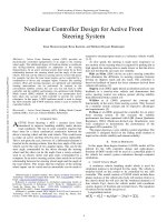
well-posed. Figure 2.1 depicts the pulse input and the resulting output response.
It is noticed that the output response will be still significant and last for long after
the pulse disappears. We will take advantage of this feature to simplify the system
equation and carry out the parameter estimation into two steps: for a
i
and c in
the first step and b
i
and d in the second step.
To avoid using time derivatives of u(t) and y(t) in the identification of process
model, (2.1) will be converted to an integral equation. To this end, we need the
following integral notations,






I
0
f(t
0
, t) = f(t),
I
j
f(t
0
, t) =

t
t
0

τ
j−1
t
0
···

τ
1
t
0
f(τ
0
)dτ

0
dτ
1
···dτ
j−1
, j ≥ 1,
(2.3)
where τ
i
, i = 0, . . . , j−1 are dummy variables for relevant integrals. In the first step
of our identification, we select one fixed time point t
1
with t
1
> d + T. Integrating
Chapter 2. Process Identification from Pulse Tests 12
0
y
0
0
u
T
h
Ingegral interval
for 1st step
Integral interval
for 2nd step
T+d
t
M

t
N+1
d t
2
t
N
t
1
Figure 2.1. Rectangular pulse response and input.
(2.1) from t
1
to t > t
1
n times yields
n−1

k=0
a
k
I
n−k
y(t
1
, t) + y(t) −
n−1

k=0
α
k
(t −t

1
)
k
k!
=
m

k=0
b
k
I
n−k
u(t
1
−d, t −d) +
c(t −t
1
)
n
n!
,
(2.4)
where α
i
are related to process initial conditions at t
1
. Since t > t
1
> d + T , the
input is always zero. We have

I
j
u(t
1
− d, t −d) = 0, j = 0, ··· , n − 1. (2.5)
Substituting (2.5) into (2.4), we obtain
φ
T
1
(t)β = γ
1
(t), (2.6)
where
φ
T
1
(t) = [
−I
1
y(t
1
, t) ··· −I
n−1
y(t
1
, t) −I
n
y(t
1
, t) 1 (t − t

1
) ···
(t−t
1
)
n
n!
],
γ
1
(t) = y(t),
and
β = [
a
n−1
··· a
1
a
0
α
0
α
1
··· c
]
T
.
Chapter 2. Process Identification from Pulse Tests 13
One invokes (2.6) for t = t
i

, i = 2, . . . , N, to form
Γ
1
= Φ
1
β
where Γ
1
= [γ
1
(t
2
), . . . , γ
1
(t
N
)]
T
, and Φ
1
= [φ
1
(t
2
), . . . , φ
1
(t
N
)]
T

. t
i
, i = 1, . . . , N,
are chosen to meet t
1
< t
2
< . . . < t
N
, where N > 2n + 2. The least-squares
method is applied to get,
ˆ
β =

Φ
T
1
Φ
1

−1
Φ
T
1
Γ
1
, (2.7)
which gives the estimates for α
i
, c and a

i
.
In the second step, we integrate (2.1) in a reverse way from t
1
to t, with d <
t < T + d, n times and this will still lead to (2.4). But, for d < t < d + T , we have
I
j
u(t
1
− d, t −d) = h
(t −d −T )
j
j!
. (2.8)
Substituting (2.8) into (2.4), we obtain
φ
T
2
θ = γ
2
(t), (2.9)
where
φ
T
2
= h[
1 t t
2
··· t

n
],
γ
2
(t) =
n−1

k=0
a
k
I
n−k
y(t
1
, t) + y(t) −
n−1

k=0
α
k
(t −t
1
)
k
k!
− c
(t −t
1
)
n

n!
,
and
θ = [
θ
1
θ
2
θ
3
··· θ
n+1
]
T
.
Once again, one invokes (2.9) for t = t
i
, i = N +1, . . . , M , so that the least-squares
method is applied to estimate θ. In this step, t
N+1
> t
N+2
> . . . > t
M
and
M −N −1 > n + 1. The elements of θ are related to the model parameters b
i
and
d via
θ

k
=
n

j=max(n−m,k− 1)
b
n−j
(−d −T )
j−k+1
(j − k + 1)!(k − 1)!
, k = 1, 2, ··· , n + 1. (2.10)
They are solved from k = n + 1, n, ··· , n + 1 − m, to get
b
i
=
i

j=0
(n −i + j)!θ
n+1−i+j
(d + T )
j
j!
, i = 0, 1, ··· , m. (2.11)